Data Analysis tip - How to make a population density plot
When comparing two data sets, frequently part of the analysis involves generating an xy-scatter plot. For example, to see how well the PSAP and CLAP agree, the absorption measured by these two instruments would be plotted against each other and a regression equation determined to describe the relationship. Derek has developed an R-script to make this plot, that has some additional useful features. An example of the plot is shown below. You have access to this R-script via your AER_VM in the directory /aer/prg/r/examples/density-plot.r and you can adjust this script to plot different variables and relationships.
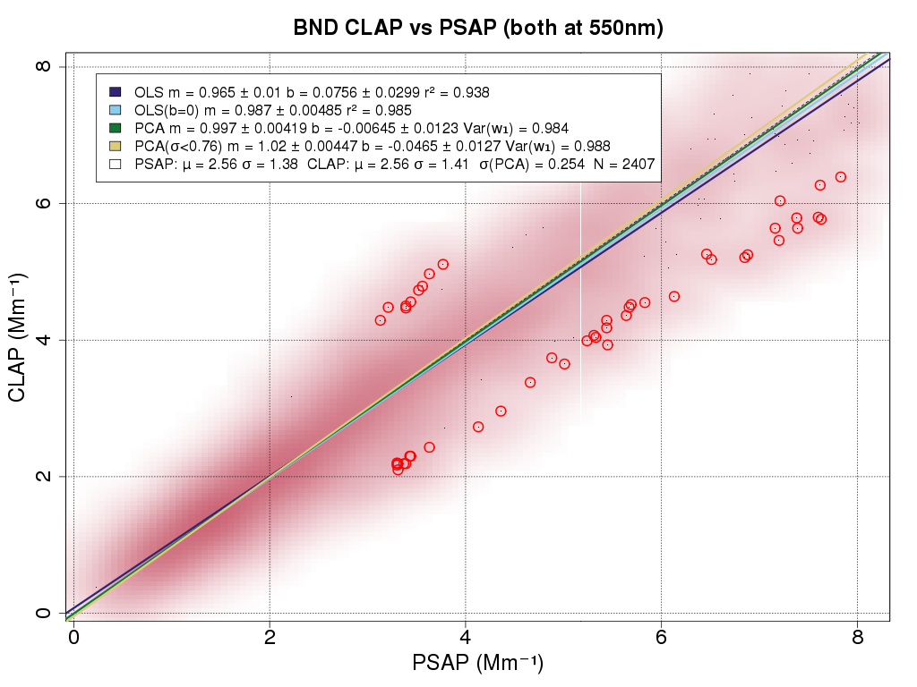
There are several features of this plot that deserve more detailed explanation.
First, it's a population density plot, so rather than seeing all the individual points (which can often hide each other) the shading gets darker in regions where there are more points. This allows identification of any groupings or patterns in the data.
Second, the legend presents four fits to the data (i) ordinary least squares (e.g., y=mx+b) (ii) ordinary least squares forced through the origin (iii) principal components analysis fit and (iv) principal components analysis filtered fit (fit with circled outliers removed). The legend also provides the mean and standard deviation for the data.
Third, the script identifies any outliers in the data which enable the user to check for issues (e.g., due to instrument malfunction) for those data points.
Pretty cool, right? So how does one actually utilize this script?
(1) Copy the script into a working directory. For example you could type:
cp /aer/prg/r/examples/density-plot.r /aer/bnd/work/2014/
and change to that working directory:
cd /aer/bnd/work/2014/
(2) Edit the script to reflect the plot you want to make. For example, at the top of the script there is a section to select the station, daterange and instruments. it looks like this:
# Parameters that specify the data to load
station <- "BND";
startTime <- "2010-12-02T02:11:58Z";
endTime <- "2011-03-28T00:00:00Z";
archive <- "avgh";
xVariable <- "BaG0_A11";
yVariable <- "BaG0_A12";
records <- "A11a,A12a";
Following that, there's a section to set the axis titles and the types of fitlines to plot. Further down there are other settings that can be changed - the script has lots of comments so potential script changes should be fairly obvious. For editing the script you can use the text editor 'nedit' or 'vi' (vi is arcane)
(3) Once you've edited the script you can run it. To run the R-script you would type:
./density-plot.r
The script will extract the data, process it and generate a plot in the directory called 'Density.png'. (If you scroll down in the R-script you will see where you can change features of the plot like the name and size and background). Note: there will only be a plot in the directory. There will not be a data file in the directory (which is really nice as it keeps things neat!)