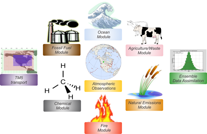
To learn more about a CarbonTracker component, click on one of the above images.
Or download the full PDF version for convenience.

Introduction

Data assimilation is a process by which observations of the 'state' of a system help to constrain the behavior of the system in time and space. An example of one of the earliest applications of data assimilation is the system in which the trajectory of a flying rocket is constantly (and rapidly) adjusted based on information of its current position to guide it to its exact final destination. Another example is weather prediction models that are updated every few hours with measurements of temperature, winds and other variables, to improve the accuracy of future forecasts. Data assimilation is usually a cyclical process; estimates are refined over time as more observations about the "truth" become available. Mathematically, data assimilation can be done with a number of techniques. For large systems, so-called variational and ensemble techniques are most successful. Because of the size and complexity of the systems studied, data assimilation projects inevitably involve supercomputers to model the known physics of a system. Success in guiding these models, often strongly depends on the number of observations available to inform on the true state of the system.

In CarbonTracker, the model that describes the system contains relatively simple descriptions of greenhouse gas emissions from anthropogenic and natural processes. In time, we alter the behavior of this model by adjusting a small set of parameters as described in the next section.

Detailed Description

Five surface flux modules drive instantaneous CH₄ fluxes in CarbonTracker-CH₄ so that the total emission of CH₄ to the atmosphere is described by:

F(x, y, t) = λ • F_natural(x, y, t) + λ • F_{fossil fuel}(x, y, t) + λ • F_{agriculture/waste}(x, y, t) + λ • F_fire(x, y, t) + λ • F_ocean(x, y, t)

Where λ represents a set of linear scaling factors applied to the fluxes (F) that are to be estimated in the assimilation. These scaling factors multiply prior estimates of methane fluxes to produce the emissions presented on the CarbonTracker-CH₄ web site. A total of 121 parameters are estimated, 10 terrestrial emission processes for 12 continental regions (corresponding to the TRANSCOM continental regions but with the addition of a tropical African region), and global fluxes from the ocean. The terrestrial emissions include anthropogenic emissions due to fugitive emissions from coal, oil and gas production; agriculture and waste emissions (rice production, for example); livestock and their waste; and emissions from landfills and wastewater. Natural emissions include contributions from wetlands, termites, uptake in dry soils and wild animals. The final terrestrial emission category is fires, and this is treated as a separate category due to the existence of strong spatial constraints coming from satellite observations of hot spots. In general, the spatial distribution of the prior flux estimates is an important constraiint on the assimilation, i.e. known location of fossil fuel production provides information to the assimilation system on whether a signal measured at a particular observation site could have a fossil fuel component. (More information on the prior flux estimates may be found here.)

A.   Ensemble Size and Localization

The ensemble system used to solve for the scalar multiplication factors is similar to that described by Peters et al. [2005], and is based on the square root ensemble Kalman filter of Whitaker and Hamill, [2002]. We have restricted the length of the smoother window to only five weeks as we found the derived flux patterns within North America to be robustly resolved well within that time. We caution the CarbonTracker users that although the North American flux results were found to be robust after five weeks, regions of the world with less dense observational coverage (the tropics, Southern Hemisphere, and parts of Asia) are likely to be poorly observable even after more than a month of transport and therefore less robustly resolved.

Ensemble statistics are created from 500 ensemble members, each with its own background CH₄ concentration field to represent the time history (and thus covariances) of the filter. To dampen spurious noise due to the approximation of the covariance matrix, we apply localization [Houtekamer and Mitchell, 1998] for non-MBL sites only. This ensures that tall-tower observations within North America do not inform on concentrations, for instance tropical African fluxes, unless a very robust signal is found. In contrast, MBL sites with a known large footprint and strong capacity to see integrated flux signals are not localized. Localization is based on the linear correlation coefficient between the 500 parameter deviations and 500 observation deviations for each parameter, with a cut-off at a 95% significance in a student's T-test with a two-tailed probability distribution.

B.   Dynamical Model

In CarbonTracker, the dynamical model is applied to the mean parameter values λ as:

λ _t^b = (λ  _t-2^a + λ  _t-1 ^a + λ  ^p  )   ⁄   3.0

where "a" refers to analyzed quantities from previous steps, "b" refers to the background values for the new step, and "p" refers to real a-priori determined values that are fixed in time and chosen as part of the inversion set-up. Physically, this model describes that parameter values λ for a new time step are chosen as a combination between optimized values from the two previous time steps, and a fixed prior value. This operation is similar to the simple persistence forecast used in Peters et al. [2005], but represents a smoothing over three time steps thus dampening variations in the forecast of λ^b in time. The inclusion of the prior term λ^p acts as a regularization [Baker et al., 2006] and ensures that the parameters in our system will eventually revert back to predetermined prior values when there is no information coming from the observations. Note that our dynamical model equation does not include an error term on the dynamical model, for the simple reason that we don't know the error of this model. This is reflected in the treatment of covariance, which is always set to a prior covariance structure and not forecast with our dynamical model.

C.   Covariance Structure

Prior values for λ^p are all 1.0 to yield fluxes that are unchanged from their values predicted in our modules. The prior covariance structure describes the magnitude of the uncertainty on each parameter, plus their correlation in space. For the current version of CarbonTracker-CH₄, we have assumed a diagonal prior covariance matrix so that no prior correlations between estimated parameters exist. The effect of this choice may be strong anti-correlations between estimated parameters in regions where few observational constraints exist; however, larger-scale aggregations of these regions are expected to yield more robust estimates. In our standard assimilation, the chosen standard deviation is 75% on all estimated parameters.

Further Reading

• Whitaker and Hamill, 2002 paper
• Peters et al., 2005 paper