SECTION II
REEVALUATION OF INSTRUMENT CONSTANTS
WALTER D. KOMHYR
This section describes procedures for determining and applying final corrections to raw observational Dobson spectrophotometer total ozone data obtained with instruments that have been periodically calibrated relative to World Standard Dobson Spectrophotometer 83 or relative to a secondary standard Dobson instrument with calibration traceable to instrument 83. The long-term ozone measurement precision of Dobson instrument 83 has been maintained to better than ±1% since 1962 [Komhyr et al., 1989]. The technique of calibrating all instruments of the global Dobson instrument network relative to instrument 83 standardizes total ozone measurements throughout the world, causing ozone data from all instruments to be directly comparable.
The correction methods described herein apply, furthermore, to Dobson instruments that have been operated according to procedures described by Dobson [1957] in the "Observers' Handbook for the Ozone Spectrophotometer" and by Komhyr [1980] in WMO Report No. 6 entitled "Operations Handbook--Ozone Observations with a Dobson Spectrophotometer." In addition to having "initial" and "final" calibrations relative to Dobson instrument 83, such instruments have had performed on them Hg lamp (wavelength-setting) tests and standard lamp tests at monthly intervals, and optical wedge re-calibrations every several years.
Data reprocessing procedures are described in the following sections for three cases. First, we consider the situation where a change occurred in the spectral characteristics of a Dobson instrument with time, but instrument optical wedge characteristics remained unchanged, and the observational data were not highly air mass (μ) dependent. Second, we treat the case where a Dobson instrument, with a well calibrated optical wedge, exhibits excessive μ-dependency in observed ozone values relative to ozone values measured simultaneously with Dobson instrument 83 or with a secondary standard Dobson instrument. Finally, procedures are described for reprocessing and correcting Dobson instrument data obtained during observing time intervals when a change occurred in the instrument's optical wedge. In the case considered, corrections are also made for an additional change in instrument spectral characteristics and, for μ-dependency in the observations.
The re-evaluated Dobson instrument data must be kept independent of other ozone data sets. Thus, ozone data from satellite instrument ozone observations, for example, should not be used in correcting the Dobson instrument data.
2.1 Use of Vigroux Ozone Absorption Coefficient Scale for Data Reprocessing
Final data processing for observations made during 1 July 1957 through 31 December 1991 should be performed using the Vigroux [1953, 1967] ozone absorption coefficient scale, with the 1.388 cm-1 absorption coefficient for AD wavelengths adopted as standard. Final results are ultimately to be archived at the WODC in Toronto, Canada, where all ozone values will be converted to the Bass-Paur [1985] ozone absorption coefficient scale as adapted for use with Dobson instruments by Komhyr et al. [1993]. The Bass-Paur [1985] ozone absorption coefficients were adopted for use throughout the world for Dobson instrument data processing beginning January 1, 1992 [Hudson et al., 1991]. On January 1, 1992, also, new improved Rayleigh molecular scattering coefficients were adopted for use for total ozone data processing [Komhyr et al., 1993]. The combined effect of the use of the new ozone absorption and molecular scattering coefficients has been to decrease ozone values by 2.6% compared to values obtained in the past.
2.2 Dobson Instrument 83 and 65 Calibration Scales
Dobson instrument 83 calibration scales, relative to which Dobson instruments have been calibrated throughout the years, are the following:
#83 June 18, 1962
#83 June 26, 1972
#83 August 26, 1976
#83 July 10, 1987
#83 August 26, 1991
Detailed information regarding slightly improved (F1) versions of these scales is presented in Appendix 2.A in the form of NA, NC, and ND tables with associated reference standard lamp readings. Except for the June 26, 1972, calibration scale, NA, NC, and ND values in the updated F1 scales are 0.004, 0.002, and 0.001 units larger, respectively, than those in the original scales, causing computed ozone values to be about 0.3% larger (at air mass ~2 and total ozone 300 DU) than values obtained using the original scales. The small scale change arose from improved calculations of μ at Mauna Loa Observatory, the site of Dobson instrument 83 calibrations, as well as from correction of a small glitch in earlier computations of Julian calendar day.
Due to an inadvertent computational error, the #83 June 26, 1972, calibration scale was originally established inaccurately. It is especially important, therefore, to correct any calibration data obtained in the past using this scale with the corrected and updated #83 June 26, 1972 F1 scale given in Appendix 2.A.
The instrument 83 calibration scales are basically interchangeable. Thus, either the #83 July 10, 1987 F1 scale or the #83 August 26, 1991 F1 scale can be used successfully in processing calibration data for a field Dobson spectrophotometer calibrated on, say, a day in 1989.
Because a number of Dobson spectrophotometers have been calibrated relative to NOAA/CMDL secondary standard Dobson instrument 65, we provide in Appendix 2.B the F1 calibration scales for instrument 65. The scales are designated as:
#65 April 10, 1981 F1
#65 May 21, 1990 F1
#65 August 30, 1991 F1.
Instrument 65 and 83 calibration scales were essentially identical through 1991 but began to diverge in 1992 causing instrument 65 ozone values to be larger than those of instrument 83 by 1%. The cause of the discrepant results is under investigation.
2.3 Data Reprocessing Procedures - Stable Dobson Instrument
Optical Wedge and No μ-Dependency in the Observations
We describe here the application of final corrections to Dobson instrument observational NA, NC, NC', and ND values obtained during a time interval when a significant change occurred in the spectral characteristics of the instrument as revealed by a "final" calibration of the instrument relative to a standard spectrophotometer, but when the instrument's optical wedge characteristics remained unchanged, and when μ-dependence was not present in the observations. (In the example to follow, some μ-dependency is present, but for purposes of illustration, we will assume it to be insignificant.). The data processing procedures described here are useful, also, for improving the quality of ozone data obtained during a time interval for which an "initial" instrument calibration relative to a standard may have lacked high precision.
Gradual changes in Dobson instrument spectral characteristics may occur, for example, due to corrosion of the instrument's cobalt filter1, contamination of the instrument's optics, or an aging photomultiplier tube. While such changes in spectral characteristics are largely compensated for by the application of monthly standard lamp test corrections during data processing, residual errors may remain. Abrupt changes in Dobson instrument jarring which may disturb instrument optical alignment, sudden optical contamination, or when partial damage occurs to the instrument photomultiplier due to inadvertent exposure to excessive light.
1This occurs in humid atmospheres when the instrument silica gel air drier is not renewed often enough.
As an illustrative example of such data reprocessing, Appendix 2.C shows "initial" and "final" calibration data for Dobson spectrophotometer 33 relative to standard instrument 83 obtained April 15, 1986, and May 11, 1988. The "initial" calibration data include newly established reference N tables and standard lamp readings dated April 15, 1986 R1. The "final" instrument 33 calibration, performed May 11, 1988, showed that mean corrections of -0.59, -0.72, and -1.79 were needed, respectively, to 100NA, 100NC, and 100ND values2 of the April 15, 1986 R1 N tables used for data processing. (These mean corrections were deduced from instrument 33 and 83 comparison ozone data obtained in the μ-range 1.15-2.5.). The correction needed to 100NAD values was, therefore, 1.21, which is significant.
2A convention is employed in expressing N values in Appendices 2.C-2.E whereby true N values are multiplied by 100.
In final processing of April 15, 1986-May 11, 1988, observational ozone data, we begin by using the reference N tables and standard lamp readings dated April 15, 1986 R1 (Appendix 2.C). For an ADDSGQP type observation, for example, correct NA and ND values are deduced from
NA = N'A + ΔNA + ΔNA(t)       (1)

ND = N'D + ΔND + ΔND(t)       (2)
Where N'A and N'D are obtained from the April 15, 1986 R1 N tables corresponding to the Dobson instrument observational dial readings RA and RD, respectively; the ΔN's are the standard lamp corrections to the N values, determined from differences in reference standard lamp N values dated April 15, 1986 R1 and N values determined by linear interpolation of routine monthly standard lamp test data; and the ΔN(t) are the time-dependent N-value drift corrections determined from the "final" calibration of instrument made May 11, 1988 (Appendix 2.C). The time dependent function to be used in applying the drift corrections may be linear, exponential, step, etc., or a combination of these. Standard lamp test history as well as other pertinent instrument information should be examined in establishing the time dependent function to use when applying the drift corrections.
The following numerical example illustrates the procedures described above for final data processing.
(a) We consider an AD-DSGQP observation made at Bismarck, North Dakota, April 3, 1987, at
18h 20m 00s UT (μ=1.339). The
observation yielded mean RA = 122.4° and mean
RD = 39.9°.
From the N tables dated April 15, 1986 R1 (Appendix 2.C) , we
obtain 100N'A = 98.1
and 100N'D = 33.4.
(b) Standard lamp corrections needed this day (not shown), determined by linear
interpolation from
lamp tests made March 29, 1987, and April 27, 1987, were
100ΔNA = -1.0 and
100ΔND = -0.7.
(c) With regard to the ΔN(t) corrections, Appendix 2.C shows that
during April 15, 1986 to
May 11, 1988, Dobson instrument 33
standard lamp N value readings changed by about two
100N units. Examination of the monthly
standard lamp test data for the instrument showed the
change to have occurred
approximately linearly with time. Therefore, using the N-value drift
correction data shown on the
last page of Appendix 2.C, and considering that April 3, 1987,
occurred 0.467 of the way into the
time interval April 15, 1986-May 11, 1988, we have that
100ΔNA(t) = 0.467(-0.59 - 0.00) = -0.276

100ΔND(t) = 0.467(-1.79 - 0.00) = -0.836
(d) Evaluating relations (1) and (2), then we have
NA = 0.981 - 0.010 - 0.003 = 0.968

ND = 0.334 - 0.007 - 0.008 = 0.319
Finally, total ozone amount for the observation, computed using Vigroux ozone absorption coefficients, is
XAD = 1000 * ((0.968 - 0.319)/(1.388 * 1.339) - 0.008) = 341 DU
Monthly standard lamp N-value corrections and the N-value calibration drift corrections should be applied not only to direct sun observational data, but also to data obtained from zenith-sky observations. Corrections to NC' values are determined from routine, monthly standard lamp tests. For standard lamp corrections to be reliable, it is important always to have operated the standard lamps at correct voltages.
2.4 Data Reprocessing Procedures - Stable Instrument Optical Wedge,
but Data Exhibiting μ-Dependency
Here we consider the situation where calibration ozone data, obtained with a spectrophotometer having a well calibrated, stable optical wedge, exhibit significant μ-dependency relative to ozone measured coincidentally with a standard spectrophotometer. Cause of the μ-dependency may be use with the instrument of an erroneous wavelength setting table; some defect in instrument optical alignment; or one or more defective optical components, e.g., a quartz prism fabricated from inferior quality quartz that attenuates ultraviolet radiation excessively, a cobalt filter with insufficient opacity at near ultraviolet wavelengths, or a corroded cobalt filter that slightly alters the effective wavelengths passing through the Dobson instrument during observations. Because the exact cause of the &mu-dependency is often difficult to determine, it is important not to over correct for it. If AD wavelength calibration ozone data for an instrument vary by less than about ±1% relative to the standard Dobson instrument ozone values for 1.15<μ<2.5, then μ-dependent corrections are most likely not worthwhile applying. Corrections may not be necessary, also, when single pair wavelength ozone observations exhibit significant μ-dependency, but double pair wavelength observations do not.
2.4.1 Observations Made on Non-Standard Wavelengths
This may occur when a Q-setting table is inadvertently established incorrectly for one or more of the Dobson instrument wavelength pairs. The standard ozone absorption coefficients, then, do not apply. However, by using more appropriate (effective) absorption coefficients, the μ-dependency in the ozone observations can be largely eliminated.
The procedure for establishing a double pair wavelength (e.g., AD wavelength) effective ozone absorption coefficient for a spectrophotometer (say, instrument 63) and calibrating it relative to a standard spectrophotometer (say, instrument 83) is as follows: Simultaneous AD-DSGQP observations are made with the two instruments during one-half day as μ varies between 1.15 and 2.5. For instrument 63 properly calibrated, we have for any observations pair
X63AD = X83AD
and
 N63AD + ΔN63AD        βAD m p          N83AD          βAD m p
----------------  -  ------------  =  ---------  -  ------------
    α63AD μ           α63AD μ p0       α83AD μ      α83AD μ p0
where
ΔN63AD = Correction needed to Dobson instrument 63 NAD values,
and
α63AD = Effective AD wavelength ozone absorption coefficient for instrument 63.
In the above relation, the two terms containing the Rayleigh scattering coefficients, βAD, are approximately equal and cancel for observations on double pair wavelengths. The relation may then be written as
A plot of N63AD vs. N83AD/α 83AD observational data yields a straight line with slope α63AD and intercept -ΔN63AD. Thus, the effective AD wavelength ozone absorption coefficient is determined for the instrument, together with the correction to the instrument's N-tables.
For single pair wavelength observations (e.g., the D wave-lengths), the Rayleigh scattering terms referred to above become significantly different, so that the above method cannot be used e.g., to determine α63D. However, α63D and corrections to N63D values can be obtained by a successive approximation method. For an instrument measuring, e.g., ozone amounts too high at low μ, ozone amounts are computed using decreased α63D and N63D values. Final α63D and N63D values are chosen that yield measured ozone amounts closely similar to those obtained with the standard instrument 83 for all μ.
2.4.2 Correcting for μ-Dependency Due to Other Causes
This section describes more general but approximate procedures for correcting for μ-dependency in ozone observations arising, for example, from light scattering within the instrument or other causes, including wavelength setting errors. As shown in section 2.5, the method can be used, if necessary, when correcting ozone data obtained with a spectrophotometer whose optical wedge characteristics changed with time.
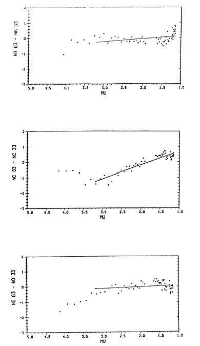
For illustration, Appendix 2.D shows "initial" and "final" calibration data for Dobson spectrophotometer 79, relative to standard Dobson instrument 83, obtained August 25, 1981, and June 19, 1985. Note that for the August 25, 1981 R1 calibration, significant μ-dependent NA-, NC-, and ND-value differences exist for instrument 79 relative to corresponding N-values for instrument 83. These are defined by the linear relations:
100ΔNA(μ)i = -27.28 + 0.9992μ + 25.51      (3)


100ΔNC(μ)i = -26.38 + 0.5846μ + 25.34      (4)


100ΔND(μ)i = -28.55 + 0.5106μ + 27.65      (5)
ΔNAD and ΔNCD differences for the two instruments on the other hand, are relatively μ-independent giving rise to μ-dependent ozone differences for instrument 79 versus instrument 83 of only ±0.5% for 1.15<=μ<=3.2.
The final calibration data for Dobson instrument 79, of June 19, 1985 (Appendix 2.D), not only show a highly significant μ-dependency in NC values relative to Dobson instrument 83 NC values but also slope reversals in the case of the instrument 79 μ-dependent NC and ND values compared to corresponding results obtained in 1981. Again, ΔNAD differences for the two instruments are relatively independent of μ, but ΔNCD differences are highly μ-dependent, causing instrument 79 XCD values to be underestimated by 4.7% at μ = 1.33 but overestimated at μ = 2.85 by 1.9%. As shown in Appendix 2.D, the μ-dependency in the instrument 79 calibration data of June 19, 1985, is defined by
100ΔNA(μ)f = 0.7067 - 3.5786μ + 1.1641μ2 - 0.0903μ3 (6)100ΔNC(μ)f = -0.1559 + 2.4719μ - 2.5068μ2 + 0.4657μ3 (7)
100ΔND(μ)f = -5.3086 + 10.2567μ - 5.1692μ2 + 0.7756μ3 (8)
Final processing of ozone data obtained with Dobson instrument 79 during August 25, 1981-June 19, 1985, is performed using the August 25, 1981 R1 N tables and reference standard lamp data given in Appendix 2.D. To process an observation made, for example, on A and D wavelengths, first convert observed mean RA and RD (instrument dial reading) values to N'A and N'D values where the primes indicate (as in section 2.3) that additional N-value corrections are needed. Then apply standard lamp corrections ΔNA and ΔND to these values based on monthly standard lamp tests as described in section 2.3. Corrected NA and ND values for the observation are then obtained from
NA = N'A + ΔNA + ΔNA(μ,t)                                (9)

ND = N'D + ΔND + ΔND(μ,t)                                (10)
where ΔNA(μ, t) and ΔND(μ, t) are needed additional μ and time dependent N-value corrections.
Information on how the μ-dependent N-value correction changed with time must be gleaned from an examination of the instrument's standard lamp test history and other relevant instrument information. For the purpose of illustration, we assume here that the change occurred approximately linearly with time and independently of measured total ozone. We have then
ΔNA(μ,t) = ΔNA(μ)i + r(ΔNA(μ)f - ΔNA(μ)i)    (11)

ΔND(μ,t) = ΔND(μ)i + r(ΔND(μ)f - ΔND(μ)i)    (12)
when r is the fraction of time that elapsed on the day of the observation since August 25, 1981, within the observing time interval under consideration.
The following numerical example illustrates the procedures described above for final data processing.
(a) We consider an AD-DSGQP observation made at Nashville, Tennessee, June 29, 1983
at 18h, 19m, 00s UT (μ = 1.033). The observation yielded mean
RA = 96.9° and RD
= 51.3°.
From the N tables dated August 25, 1981 R1
(Appendix 2.D) we obtain, corresponding to the
instrument dial readings,
100N'A = 67.9 and 100N'D = 22.1.
(b) Corrections (not shown) needed on June 29, 1983 to N values, based on monthly
standard lamp
test data, were 100ΔNA = 3.0 and
100ΔND = 2.4.
(c) Evaluating relations (3), (5), (6), and (8) above for μ = 1.033 to obtain
the needed μ-dependent
N-value corrections, we have
100ΔNA(μ)i = -27.28 + 1.032 + 25.51 = -0.738

100ΔND(μ)i = -28.55 + 0.527 + 27.65 = -0.373

100ΔNA(μ)f = 0.7067 - 3.6967 + 1.2422 - 0.0995 = -1.847

100ΔND(μ)f = -5.3086 + 10.5952 - 5.5160 + 0.8549 = 0.626
(d) For the observation made June 29, 1983, the fraction of time, r, that
elapsed since August 25, 1981
within the time interval August 25, 1981-June 19, 1985,
is 0.483. Evaluating relations (11)-(12)
we then have
ΔNA(μ,t) = -0.0074 + 0.483(-0.0185 + 0.0074) = -0.013

ΔND(μ,t) = -0.0037 + 0.483(0.0063 + 0.0037) = 0.0011
(e) Relations (9) and (10) are then evaluated to yield
NA = 0.679 + 0.030 - 0.013 = 0.696

ND = 0.221 + 0.024 + 0.001 = 0.246
Finally, total ozone amount for the amount observation, computed using Vigroux ozone absorption coefficients, is
XAD = 1000[(0.696 - 0.246)/(1.388 * 1.033) - 0.009] = 305 DU
The method described above for final processing of μ-dependent observational ozone data involves N-value determinations from "initial" calibration mean N tables (derived from instrument 79 and 83 comparison calibration observations made at 1.15<μ<2.5) to which are added μ-dependent N-value corrections. An alternate procedure, yielding equivalent results, would be to use, instead, μ-dependent N tables comprised of G tables with associated μ-dependent ΔG values that convert the G tables to N tables. For the example considered, the μ-dependent ΔG values are defined by the three linear relations that appear on the top of the third page of Appendix 2.D.
2.5 Data Processing Procedures - Unstable Dobson Instrument Optical Change in Instrument Spectral Characteristics, and μ-Dependency in the Observations
We finally consider the situation where, during a certain time interval, a change occurred in the Dobson instrument optical wedge characteristics. Here it is assumed that a reasonable estimate can be made of how the wedge changed with time, whether linearly, exponentially, or via a step function, etc.; and that optical wedge calibrations and instrument calibrations relative to a standard spectrophotometer were performed prior to and after the time interval of the wedge change. With such information, it is possible to improve reprocessed ozone data quality not only by largely accounting for the optical wedge change but also by substantially correcting for additional long-term instrument calibration drift that may have occurred due to causes described in sections 2.3 and 2.4 as well as for μ-dependency in the observations.
As an illustrative example, we consider total ozone data obtained at Nashville, Tennessee, with Dobson instrument 79 between September 10, 1975 and August 14, 1981. During this time interval the spectral characteristics of the optical wedge in instrument 79 changed significantly by up to about 0.035 unit, as indicated in Table 1 (below).
 Table 1. Optical Wedge Density Changes for Dobson
         Instrument 79 During September 9, 1975-August 24, 1981.

----------------------------------------------------------------------
 Inst. Dial
Readings (°)    GA 1981-GA 1975    GC 1981-GC 1975    GD 1981-GD 1975
----------------------------------------------------------------------

      10             0.002              0.000              0.001
      50            -0.005             -0.005             -0.006
     100            -0.018             -0.017             -0.018
     150            -0.021             -0.022             -0.021
     200            -0.030             -0.033             -0.032
     250            -0.033             -0.037             -0.032
     290            -0.029             -0.035             -0.032
----------------------------------------------------------------------
For final data processing, it is necessary to adopt some functional form for the temporal optical wedge density changes. As much available information as possible should be used in deciding on what functional form to adopt. We begin by examining standard lamp test data for Dobson instrument 79 (Figure 1). Here standard lamp 79C readings appear to be relatively constant during September 29, 1975-March 31, 1979, but then increase with time through August 14, 1981. Such data imply that the change in optical wedge densities may have begun about April 1, 1979, and proceeded in a linear fashion through 1981. But additional data suggest a different scenario. Examining all available calibration data (not shown) for instrument 79, we find that for the time interval defined by instrument 79 optical wedge calibration dates of July 23, 1962; July 7, 1971; October 17, 1973; September 9, 1975; August 24, 1981; and June 27, 1985, the optical wedge density rates of change were 0% yr-1, 0.2% yr-1, 0.6% yr-1, 0.5% yr-1, and 0.3% yr-1, respectively. (These were determined from optical wedge density data for instrument 79 R-dial readings of 200°, and are assumed to be representative of density change rates throughout the wedge.) Thus the conclusion must be that instrument 79 optical wedge density characteristics changed approximately linearly throughout the entire observing interval under consideration, namely, September 10, 1975-August 14, 1981. What then caused the change in the character of the standard lamp readings beginning about April 1, 1979 (Figure 1)?
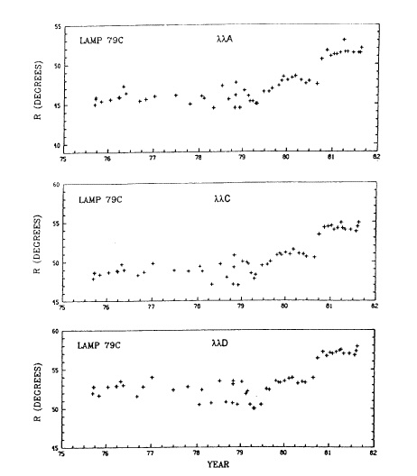
Figure 1. Standard Lamp 79C test data for Nashville Dobson instrument 79 obtained
during September 1975-August 1991.
Our historical records show that in August 1981, when instrument 79 was received in Boulder, Colorado, the cobalt filter in front portions of the filter exhibiting a milky coloration. As indicated previously, filter corrosion occurs in humid air. (In 1975 the filter exhibited no sign of corrosion.) We surmise, therefore, that following about April 1, 1979, silica gel air drier within the instrument was not renewed often enough to keep the instrument dry. As a result, instrument 79 optical characteristics changed approximately linearly with time during April 1, 1979-August 24, 1991, due to cobalt filter deterioration.
In final processing of the total ozone data obtained at Nashville we, therefore, take the spectral characteristics of Dobson instrument 79 to have changed in part linearly with time during September 9, 1975-August 24, 1981, due to optical wedge density changes, and additionally linearly with time during April 1, 1979-August 24, 1981, due to cobalt filter deterioration. Final data processing should therefore, proceed as follows, where corrections are also made for μ-dependency in the instrument 79 observational data that were partly induced by the cobalt filter corrosion.
Appendix 2.E presents "initial" calibration data for Dobson instrument 79 relative to Dobson instrument 83 obtained September 19, 1975. Instrument 79 optical wedge density tables used in analyzing the calibration data were those determined September 9, 1975. Note (Appendix 2.E) that the calibration data for instrument 79 exhibit little μ-dependency relative to instrument 83 data. The new calibration scale for Dobson instrument 79, dated September 10, 1975 R1, is presented in Appendix 2.E.
A "final" calibration of instrument 79 was conducted in Boulder on August 14, 1981. Appendix 2.E presents usual analysis data for the instrument comparison where standard lamp corrections to the data are applied and a change in instrument 79 calibration relative to its calibration of September 19, 1975 R1, is determined. (No account is taken here of instrument 79 optical wedge density changes.) Note (Appendix 2.E) the large instrument 79 calibration change (i.e., ΔNAD = 0.0244) that occurred during September 10, 1975-August 14, 1981, that was not corrected for by the application of standard lamp test data. This calibration change corresponds to AD-DSGQP ozone measurement errors on August 14, 1981, of 5.6% at μ = 1, and 2% at μ = 3. A large calibration change is evident, also, for CD wavelength observations made with instrument 79.
In Appendix 2.E the instrument 79 "final" calibration data of August 14, 1981, are processed using correct optical wedge density data, determined August 24, 1981. When processing the data, GA and GD values in the tables corresponding to instrument 79 observational RA and RD R-dial readings, respectively, are converted to N'A and N'D values3 using the relations
N'A = GA + (NAS - GAS)             (13)

N'D = GD + (NDS - GDS)             (14)
where GAS and GDS are the G values obtained from the G tables dated August 24, 1981, corresponding to reference standard lamp readings RAS and RDS obtained August 14, 1981; and NAS and NDS are the reference lamps N values established September 10, 1975 (Appendix 2.E). In practice, mean results of tests with two or more reference standard lamps are used for the N-value determinations. For the example under consideration, mean NAS - GAS = -0.292 and mean NDS - GDS = -0.304 were computed from tests made August 14, 1981, with instrument 79 reference standard lamps 79C and 79D (Appendix 2.E).
3Primes associated with NA and ND values indicate that additional corrections to these values may be needed.
Results of processing of the instrument 79 "final" calibration data of August 14, 1981, are summarized in Appendix 2.E. Note that use of correct optical wedge densities in the data processing has reduced former mean NAD and NCD calibration error of -0.0244 and -0.0099 (Appendix 2.E) to -0.0120 and -0.0035, respectively. We interpret the residual error to have resulted from Dobson instrument 79 spectral characteristics changes due to cobalt filter deterioration. Note that the errors exhibit a μ-dependency, part of which was an original spectral characteristic of Dobson instrument 79, but part of which was induced by the cobalt filter corrosion.
In reprocessing total ozone observational data (i.e., applying final corrections to the data) for example, for an AD-wavelength observation, it is first necessary to evaluate relations (13) and (14). Here the standard lamp NAS and NDS values are constants (Appendix 2.E), while the GAS and GDS values are derived for the day of the total ozone measurements from linear interpolation of monthly standard lamp test RAS and RDS values, as well as from the G-tables dated September 9, 1975, and August 24, 1981. The GA and GD terms in relations (13) and (14), corresponding to mean RA and RD values for the ozone observation, are also derived by linear interpolation from the September 9, 1975, and the August 24, 1981, G-tables. N'A and N'D values thus computed from (13) and (14) for the AD-wavelength observations are corrected for temporal drift of the optical wedge densities of Dobson instrument 79, but they are not corrected for the change in instrument 79 spectral characteristics that occurred during April 1, 1979-August 24, 1981, due to cobalt filter deterioration, including μ-dependency. Denoting these additional, time dependent corrections by ΔNA(μ,t) and ΔND(μ,t), we have
NA = N'A + ΔNA(μ,t)        (15)

ND = N'D + ΔND(μ,t)        (16)
where the NA and ND values are now corrected not only for the optical wedge calibration drift, but also for the cobalt filter deterioration effects as well as for observational time-dependent μ-dependency.
As indicated earlier, a small μ-dependency in instrument 79 ozone observations relative to instrument 83 ozone observations is evident in the "initial" calibration of instrument 79 on September 10, 1975 (Appendix 2.E). While a μ-dependency of this magnitude would not normally be considered for correction, we account for it here mainly to demonstrate the technique. As shown in Appendix 2.E, applicable μ-dependent corrections for Dobson instrument 79 September 10, 1975, were
ΔNA(μ)i = A + Bμ - GA             (17)

ΔND(μ)i = A + Dμ - GD             (18)
where A, B, C, and D are constants, and the GA and GD are mean G-values deduced from the comparison observations made at 1.15<μ<2.5 that, when added to the G tables dated September 9, 1975 convert them to N-tables dated September 10, 1975. These linear relations4 express N-value differences as a function of μ for Dobson instruments 79 and 83 on September 10, 1975. They are assumed to be independent of total ozone amount, and to remain unchanged during September 10, 1975-March 31, 1979, the time interval when standard lamp test data for instrument 79 remained relatively constant.
4For other instrument calibrations, these relations may be parabolic or cubic.
"Final" calibration data of August 14, 1981 (Appendix 2.E), with optical wedge density drift corrected, show a change in instrument 79 spectral characteristics, including a change in the μ-dependency of the comparison observations. Applicable μ-dependent N-value corrections on this day (Appendix 2.E) are shown to be
ΔNA(μ)f = E + Fμ                   (19)

ΔNA(μ)f = J + Kμ                   (20)
where, again, E, F, H, and K are constants.
During final data processing, then, two time intervals must be considered in applying the above N-value corrections to observational data. For ozone observations made during September 10, 1975-March 31, 1979, when instrument spectral characteristics appear to have remained constant (except for the wedge density change that has been accounted for), correct observational N-values [relations (13) and (14)] are given by
NA = N'A + ΔNA(μ)i                (21)

ND = N'D + ΔND(μ)i                (22)
For the time interval April 1 to August 14, 1979, on the other hand, the μ-dependent corrections are assumed to have changed linearly with time from those given by (17) and (18) to those given by (19) and (20). Thus for ozone observations made during this latter time interval, correct N-values for an ozone observation are given by
NA = N'A + ΔNA(μ)i + r[ΔNA(μ)f - ΔNA(μ)i]                  (23)

ND = N'D + ΔND(μ)i + r[ΔND(μ)f - ΔND(μ)i]                  (24)
where r is the fraction of time that has elapsed for the particular ozone observation since April 1, 1979, within the time interval under consideration.
The following numerical example illustrates the procedures described above for final data processing:
(a) We consider an AD-DSGQP observation made at Nashville,
Tennessee, June 15, 1980, at 20h 00m 00s UT (μ = 1.171).
The observation yielded mean RA = 112.0° and mean RD = 57.2°.
From the wedge density tables dated September 9, 1975
(Appendix 2.E) we obtain, corresponding to these instrument
dial readings, 100GA = 110.5 and 100GD = 56.0. But from the
August 24, 1981, wedge density tables (Appendix 2.E) we
obtain 100GA = 108.7 and 100GD = 55.3. Now the time
interval September 9, 1975-June 15, 1980, comprises 0.799 of
the overall time interval (September 9, 1975-August 24,
1981) under consideration. Therefore, by linear
interpolation, G values corresponding to the AD-DSGQP
observational R values are 100GA = 109.1 and 100GD = 55.4.
(b) Standard lamp tests were performed on instrument 79 at
Nashville with lamps 79C on May 30, 1980, giving RAS and RDS
values of 47.6° and 53.4°, respectively; and on June 25, 1980,
giving RAS and RDS values of 47.9° and 53.5°,
respectively. By linear interpolation, we take the standard
lamp readings to be RAS = 47.8° and RDS = 53.5° on June 15,
1980. From the September 9, 1975-August 24, 1981, G tables,
corresponding G-values are found by linear interpolation to
be 100GAS = 47.8 and 100GDS = 51.9 on June 15, 1980.
Standard lamp 79C N-values are 100NAS = 22.3 and 100NDS =
25.4 (Appendix 2.E).
(c) Using relations (13) and (14) we obtain for the AD-DSGQP
observation of June 15, 1980
N'A = 1.091 + (0.223 - 0.478) = 0.836

N'D = 0.554 + (0.254 - 0.519) = 0.289
Incorporated into the N' values are corrections for
instrument 79 optical wedge density drift, but not
corrections for instrument 79 spectral characteristics
change due to cobalt filter deterioration, including μ-
dependent corrections.
(d) To correct the observational data for the additional instru-
ment spectral characteristics changes, we begin by
evaluating relations (17) - (20) above (see Appendix 2.E) for
μ = 1.171
     100ΔNA(μ)i = -24.5148 + 0.8356(1.171) + 23.03 = -0.506
     100ΔND(μ)i = -26.5822 + 0.5610(1.171) + 25.59 = -0.335
     100ΔNA(μ)f = -3.4037 + 1.2064(1.171) = -1.991
     100ΔND(μ)f = -0.5166 + 0.2543(1.171) = -0.219
(Note that had the ozone observation been made prior to
April 1, 1979, only relations (17) and (18) would have had
to have been evaluated.)
For the observations made June 15, 1980, the fraction of
time, r, elapsed since April 1, 1979, within the time
interval April 1, 1979-August 14, 1981, is 0.509. Final,
corrected N-values for this ozone observation are then
computed from (23) and (24):
     NA = 0.836 - 0.005 + 0.509(-0.020 + 0.005) = 0.823
     ND = 0.289 - 0.003 + 0.509(-0.002 + 0.003) = 0.287
(e) Total ozone amount for the observation, using Vigroux ozone absorption coefficients, is then
XAD = 1000[(0.823 - 0.287)/(1.388 * 1.171) - 0.009] = 321 DU
As in section 2.4, a variation of the data reprocessing described above, yielding equivalent results, would involve direct use of μ-dependent G tables. Such a procedure may be more adaptable to use with existing Dobson instrument data processing software than that described.
The optical wedge of Dobson instrument 79 was manufactured by R. and J. Beck, Ltd., of Oxford, England. Canada balsam cement was used in gluing the wedge sections together. Over the years, experience has shown that the cement in such wedges ages with time, causing optical densities along the wedge to change. Many of the Dobson instruments in the global network have been retrofitted with "air-space" wedges from which the cement has been removed [Komhyr and Grass, 1972]. Such wedges are inherently more stable. Nevertheless, their optical characteristics may still change with time should they become contaminated; for example, with lubricant from the optical wedge track or from the instrument optical shutter bearing.
The example presented in this section of Dobson instrument performance degradation due to cobalt filter corrosion by humid air attests to the importance of keeping the Dobson instrument optics clean and dry at all times.
2.6 Air Mass Dependence of Ozone Measurements in Polluted Air
An important source of ozone measurement error is stray light interference, particularly at the shorter wavelength of the Dobson spectrophotometer A-wavelength pair. Stray light is radiation scattered by the atmosphere in the instrument's field of view, as well as unwanted radiation scattered within the instrument. The stray light effect varies among Dobson instruments [Olafson and Asbridge, 1981; Basher, 1982], significantly limiting the accuracy of AD wavelength direct sun observations at air mass (μ) values above 2.5 to 3. G.M.B. Dobson [Walshaw, 1975] examined both sources of stray light, describing a detailed investigation of errors in ozone measurements made at low sun. Basher [1982] modeled instrumental and atmospheric factors influencing stray light, including the effect of ozone amount variations. Degórska and Rajewska-Wiech [1989] showed that the stray light is influenced by local pollution--a topic that is the focus of this section. One of the methods of testing a spectrophotometer for stray light is to take a series of observations on the rising or setting sun and compare results with the stray light model of Basher [1982]. A parameter of Basher's heterochromatic stray light model is RO which depends inversely on the quality of the instrument stray light rejection properties. Values of RO were estimated to range from 10-5 to 10-3. Values of a second model parameter, a, representing the atmosphere relative attenuation of the stray light band, range from about 0.7 to 1.2 depending on ozone amount.
Figure 2 shows two sets of μ-dependent ozone data obtained with Dobson instrument 84: at Belsk, Poland in 1981 in polluted air, and at Arosa, Switzerland in 1986 in clean air. Note that in polluted air in Belsk, measured ozone decreased rapidly at μ values greater than 2.5. At Arosa, in clean air, significant decrease in ozone began at μ greater than 3.5.
The observational data in Figure 2 have been fitted with Basher model curves having the same RO values for both days, but different values of a (1.2 and 0.7). Differences in the shapes of the curves, stemming from use of the different parameters a, cannot be attributed to ozone amount differences, since ozone on both days was nearly the same (~305 DU). Thus the differences must stem from pollution effects.
In re-evaluating Dobson instrument total ozone data, it is important to know that atmospheric pollution (including turbidity) adversely affect ozone measurements at the higher μ values. Unless ozone data from series of observations at extended μ values exist for a particular station, correction for pollution effects will be difficult to make. New measurements can provide data that may be useful in assessing errors in observations made in the past. Where possible, data selected for archiving, as representative of local apparent noon, should be restricted to observations made at 1.3<μ<2, since stray light and other instrumental problems tend to degrade, also ozone measurements at low μ.
2.7 CD-Wavelength observations on Direct Sun
AD-DSGQP observations are fundamental; data from all other kinds of observations must ultimately be reduced to their calibration level. But as noted in the previous section, stray light errors, due either to instrumental factors or to sky conditions, degrade the quality of the AD-DSGQP observations at μ values larger than 2.5 to 3.
Instrumental stray light effects are less severe for the longer wavelength and more intense CD-DSGQP observations. In relatively clean atmospheres, these observations can be extended to μ values of 3.5 to 4.0. Nevertheless, because relative intensity differences for C and D wavelengths are considerably smaller than for A and D wavelengths, it is more difficult to calibrate and maintain in calibration a Dobson instrument at CD wavelengths. For stations at latitudes that must resort to CD type direct sun observations during certain times of the year, then, it is necessary to maintain an ongoing program of comparison AD-DSGQP and CD-DSGQP observations. These should be made in the μ-range 1.5 to 2.5 or 3, depending on the optical condition of the instrument, sky turbidity, and total ozone amount. In final data processing, ratios of the comparison total ozone amounts, plotted as a function of μ, should be used in correcting the CD-DSGQP observations data.
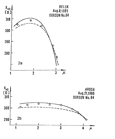
Figure 2. (a) Comparison of experimental data with stray light model: For the solid
lines, RO = 10-3.8, for the dotted lines RO = 10-4.0, a = 1.2. (b) As in (a),
but for a = 0.7.
AD-DSFI and CD-DSFI ozone measurements can be made in the μ intervals 2.5-4.0 and 2.5-6.0, respectively [Komhyr, 1980], extending the μ-range of Dobson spectrophotometer direct sun observations. This is possible because focused image observations reduce the amount of skylight entering the instrument and at the same time increase the intensity of the direct solar radiation entering the instrument. Correction procedures for both skylight and scattered light, when the focused image method is used, have been described by Hamilton [1964]. Focused image observations are, however, difficult to make requiring considerable skill by the observer. S.H.H. Larsen, University of Oslo, Norway, has adapted the methodology of Hamilton [1964] to C-DSGQP and CD-DSGQP observations which are considerably easier to make (see Appendix 2.F). Under good observing conditions, ozone measurements can be extended by this method to μ values as high as 8. Such observations are useful especially in late fall and early spring at high latitudes when solar elevation is low during the day.
2.8 Use of Empirically Established Charts for Processing Zenith Sky Observations
Zenith-sky observational data are reduced by means of empirically constructed charts that relate instrument N-values, μ, and total ozone, X. Such charts are drawn up using quasi-simultaneously obtained data from AD-DSGQP observations and observations on the clear or cloudy zenith. Nearly simultaneous direct sun and clear zenith sky observations are readily obtainable. However, when the sky is cloudy, it often becomes necessary to compare direct sun and cloudy zenith observations that have been made several hours apart.
Charts for reducing ozone measurement data from zenith sky observations, derived from observations made at Oxford, England [Dobson, 1957], were available in the past from the manufacturer of the Dobson instruments (R.J. Beck, Ltd.). Another set of charts has been published in WMO Report No. 6 [Komhyr, 1980]. They were devised in the late 1950s and early 1960s from observations made at Edmonton and Moosonee, Canada [Kinisky, 1961; Komhyr, 1961]. It is important to note that these charts cannot be used universally since the shapes of the chart curves are a function of the ozone vertical distribution, earth albedo, atmospheric clarity, and instrumental factors. Therefore, although the charts serve as useful starting tools for preliminary reduction of data, it is necessary at each station to obtain a sufficient number of comparison direct sun and zenith-sky observations to correct the charts so that they yield optimum quality data for that location.
An interesting variation of the standard method employed in constructing the zenith sky charts has been described by Hassan [1982] who used a multiple linear regression technique involving pair XDSAD and NZBLL observations to construct sky charts for Cairo, Egypt. More work is needed, however, to ascertain whether such charts can be used successfully at higher latitude stations.
Zenith sky charts can also be derived from theoretical calculations based on multiple scattering in a purely molecular atmosphere [Mateer et al., 1977]. Such calculations take into account standard or climatological ozone profiles, the effect of temperature on ozone absorption coefficients, and ground albedo. Stamnes et al. [1990] used a comprehensive radiative transfer algorithm to draw zenith sky charts. The method allows taking into consideration atmospheric optical depth and cloud height as well. Such theoretically derived charts, however, need on-site correcting to account for modelling uncertainties and instrumental factors.
Final processing of ozone observations made on zenith sky should be performed with corrected and re-drawn charts. An alternative procedure is to determine corrections; for example, to the charts provided in WMO Report No. 6, by plotting AD-DSGQP versus ADZB, ADZC, CC'ZB, CC'ZC, CDZB, CDZC observations as a function of μ. As an example, such corrections for ADZB type observations, determined at Bismarck from measurements made during 1962 to 1985, are shown in Figure 3. Ideally, such plots should be made for low, medium, and high values of ozone. Figure 4 shows similar comparison data for AD wavelength zenith cloud observations. Here the scatter in the data is considerably greater since the comparison observations were often made several hours apart during which time significant changes in ozone sometimes occurred. Cloud observations are, also, inherently less precise than are the clear zenith observations.
We have strong indication from Umkehr observations that stratospheric aerosols from occasional volcanic eruptions influence UV flux ratios emanating downward from the zenith sky at the A, C, and D Dobson instrument wavelength pairs. The extent to which these aerosols affect total ozone data derived from zenith sky observations requires further study.
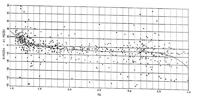
Figure 3. Corrections needed to Chart AD of WMO Report No. 6 when
processing total ozone data obtained at Bismarck, North Dakota, from
observations made on the clear zenith sky.
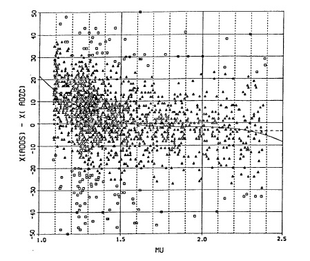
Figure 4. Corrections needed to Chart AD of WMO Report No. 6 for processing
total ozone data at Bismarck, North Dakota, from observations made
on the cloudy zenith sky.
Special attention is called to Chart NC' used in reducing CC'ZC observations. The abscissa values for this chart are fixed by setting the ΔN = 0 correction curve at the extreme right of plotted NC' values derived from observations on the blue sky. This is shown, for example, in Figure 5, for observations made a Bismarck during June 2, 1976-May 28, 1980. Should similar observational data not be available for the following several-year observing interval beginning May 29, 1980, for which new reference N tables and standard lamp readings are established for routine total ozone data reduction, the NC' chart derived from the 1976-1980 observations can continue to be used beyond May 28, 1980. However, before using it, it is first necessary to shift the ΔN=O curve of Figure 4 horizontally by the difference in reference standard lamp NC' readings for the June 2, 1976, and May 29, 1980, instrument calibrations. For example, as shown in Figure 5, the abscissa value for the curve ΔNC = 0 at μ = 1 is 100NC' = 147. If the reference standard lamp NC' values for the instrument in-the-mean are larger on May 29, 1980, by 6 100N units than they were June 2. 1976, the curve should be shifted to read 100NC' = 147 + 6 = 153 at μ=1. The need for this shift arises because Dobson spectrophotometer calibrations relative to a standard are performed at A, C, and D wavelengths, but not C' wavelengths, and NC' values are obtained from NC tables.
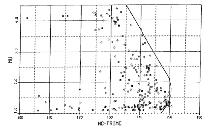
Figure 5. Illustration, from observations made at Bismarck during June 1976-
May 1980, of the method of fixing the abscissa value of the ΔN = 0
curve of the cloud correction Chart C' given in WMO Report No. 6.
The above technique may be used also when a replacement spectrophotometer, for which an NC' chart has not been established observationally, is temporarily used at a station.
2.9 Total Ozone Measurement Interfering Absorbing Species
Komhyr and Evans [1980] identified a number of trace gas species that possess absorption spectra in the spectral region of the Dobson instrument wavelengths of these, SO2 and NO2 have the greatest potential for causing Dobson instrument total ozone measurement errors. De Backer and De Muer [1991] and De Muer and De Backer [1992] have shown that in certain regions of the globe SO2 pollution may also have a significant effect on the determination of ozone trends.
Although SO2 measurements are possible with a Dobson spectrophotometer, such observations are seldom made. Near ground-level SO2 data are available in some locations from pollution monitoring networks; however, translating surface SO2 concentrations to atmospheric total column SO2 entails considerable research that is best reserved for special studies, with formal publication of results obtained in the open literature. Thus, re-evaluation of Dobson instrument data should, in general, not include correcting the data for SO2 interference or other interfering absorbing species.
An exception exists where a Dobson instrument observatory is located fairly close to a coal- or oil-fired power plant. On occasion when the observatory is downwind from the plume, measured ozone values may be too high by 10% or more. Successive ozone observations made under such conditions generally yield erratic data with a large standard deviation associated with the mean. Such data, if included in the ozone daily means archive, should be flagged as most likely being unreliable.
(For reasons given above, the re-evaluated Dobson instrument data should, also, not be corrected for changes in effective Dobson instrument ozone absorption coefficients that vary seasonally or on a secular basis as stratospheric temperatures change.)
2.10 Calibration of Dobson Spectrophotometers With Calibrated Traveling
Standard Lamps
At the 1977 International Comparison of Dobson Ozone Spectrophotometers held in Boulder, Colorado, a traveling standard lamp method was devised [Komhyr et al., 1981] for identifying Dobson instruments that have gross calibration errors. (Traveling standard lamps are calibrated with World Primary Standard Dobson Spectrophotometer 83.) Tests on 14 instruments at that time, well calibrated on a relative scale (i.e., newly optically aligned, and with high quality wavelength-setting and optical wedge calibrations), showed that such instruments can be calibrated with lamps to yield ozone measurement uncertainties at the 95% interval confidence level of 2.2%, 1.1%, and 0.7% when measuring 300 DU ozone at air mass values of 1, 2, and 3, respectively. (These errors are about twice as large as those associated with direct spectrophotometer intercalibrations.) Subsequently, seven standard lamp units were built and calibrated, each consisting of two calibrated lamps and a stable power supply.The global Dobson instrument network was then divided into seven areas, each containing from 5 to 17 instruments, and a lamp unit was shipped to each area for use in checking the calibrations of the Dobson instruments in that area. Results of the first round robin of such calibrations, conducted in 1981-1983 [Grass and Komhyr, 1985], showed that 21 of the 78 instruments tested needed re-calibration, with 17 instruments having large calibration errors of 3-10%. A second series of tests in 1985-1987 involving 81 instruments [Grass and Komhyr, 1989] showed that 13 needed re-calibration, with 5 instruments having calibration errors as large as 3-5%. A third such Dobson instrument test series, initiated in 1990, is nearing completion.
The main purpose of the traveling standard lamp tests has not been to calibrate Dobson instruments, but to check on how well they are calibrated. Such calibrations, however, can be useful when performed on instruments that are well aligned optically and have high quality wavelength-setting and optical wedge calibrations. Large calibration errors can ensue, however, for instruments that have poor, not well known, optical characteristics. Total ozone data re-evaluations for such instruments should not be based on calibrations of the instruments with traveling standard lamps.
Appreciation is expressed to M. Degórska and B. Rajewska-Wiech of the Polish Academy of Sciences; D. DeMuer of the Royal Meteorological Institute of Belgium; and S.H.H. Larsen, University of Oslo in Norway for contributions to portions of the Handbook. Helpful comments and criticisms were provided also by J. Easson of the Australian Bureau of Meteorology; A. Frolov and A. Shalamiansky of the Main Geophysical Observatory in St. Petersburg, Russia; and G.K.Y Hassan of the Egyptian Meteorological Authority in Cairo.
References
Basher, R.E., Review of the Dobson spectrophotometer and its accuracy, Rep. 13,
WMO Global
Ozone Research and Monitoring Project, Geneva, 1982.
Bass, A.M. and R.J. Paur, The ultraviolet cross-sections of ozone, I. The Measurements, in
Atmospheric Ozone, edited by C.S. Zerefos and A. Ghazi,
pp. 606-610, Reidel, Dordrecht,
Boston, Lancaster, 1985.
De Backer, H. and D. De Muer, Intercomparison of total ozone data measured with Dobson and
Brewer ozone spectrophotometers at Uccle (Belgium) from January
1984 to March 1991,
including zenith sky observations,
J. Geophys. Res., 97, 20,711-20,719, 1992.
Degórska, M. and B. Rajewska-Wiech, The effect of stray light on total ozone
measurements at
Belsk, Poland, in Ozone in the Atmosphere, Proc.
Quadr. Ozone Symp. 1988 and Tropospheric
Ozone Workshop,
ed. R.D. Bojkov and P. Fabian, A. Deepak Publishing 1989, Hampton,
Virginia, 759-761, 1989.
De Muer, D. and H. De Backer, Revision of 20 years of Dobson total ozone data at Uccle (Belgium);
Fictitious Dobson total ozone trends induced by sulfur dioxide
trends, J. Geophys. Res., 97,
5921-5937, 1992.
Dobson, G.M.B., Observers' handbook for the ozone spectrophotometer, Ann. Int. Geophys.,
Year 5, part 1, 46-89, 1957.
Grass, R.D. and W.D. Komhyr, Traveling standard lamp calibration checks on Dobson ozone
spectrophotometers during 1981-83, in Atmospheric Ozone, Proc.
Quadrennial Ozone
Symposium, Halkidiki, Greece, September 3-7,
1984, ed. C.S. Zerefos and A. Ghazi,
pp. 376-380, Reidel, Dordrecht,
1985.
Grass, R.D. and W.D. Komhyr, Traveling standard lamps calibration checks of Dobson ozone
spectrophotometers during 1985-1987, Ozone in the Atmosphere,
Proc. Quadrennial Ozone
Symposium 1988 and Tropospheric Ozone
Workshop, R.D. Bojkov and P. Fabian, Eds.,
pp. 144-146,
A Deepak, Hampton, VA, 1989.
Hamilton, R.A., Determination of ozone amounts by the Dobson spectrophotometer using the
focused sun method, Q.J. Roy. Met. Soc., 90, 333-337, 1964.
Hassan, G.K.Y., Construction of empirical zenith ozone charts and tables using the multiple
regression technique, in Atmospheric Ozone, Proc. Quadrennial
Ozone Symposium, Halkidiki,
Greece, 3-7 September 1984, ed.
C.S. Zerefos and A. Ghazi, pp. 532-542, Reidel,
Dordrecht, 1985.
Hudson, R.D., W.D. Komhyr, C.L. Mateer, and R.D. Bojkov, Guidance for use of new ozone
absorption coefficients in processing Dobson and Brewer spectrophotometer
total ozone data
beginning 1 January, 1992, WMO document RDP-825,
December 18, 1991.
Kinisky, J.J., W.D. Komhyr, and C.L. Mateer, Measurements of atmospheric ozone at Edmonton,
Canada - July 1, 1957 to June 30, 1960, Canadian Meteorological
Memoirs, No. 8, Dept.
Transport, Met. Branch, Toronto,
90 pp., 1961.
Komhyr, W.D., Measurements of atmospheric ozone at Moosonee, Canada - July 1, 1957 to July 31,
1960, Canadian Meteorological Memoirs, No. 6, Dept. Transport,
Met. Branch, Toronto,
96 pp., 1961.
Komhyr, W.D., Operations handbook - ozone observations with a Dobson spectrophotometer,
Rep. 6, WMO Global Ozone Res. and Monit. Proj., Geneva, 1980.
Komhyr, W.D. and R.D. Evans, Dobson spectrophotometer total ozone measurement errors caused
by interfering absorbing species such as
SO2, NO2, and
photochemically produced O3 in polluted
air, Geophys. Res. Lett., 7, 157-160, 1980.
Komhyr, W.D., R.D. Grass, and R.K. Leonard, Dobson spectrophotometer 83: A standard for total
ozone measurements 1962-1987, J. Geophys. Res., 94(D7),
9847-9861, 1989.
Komhyr, W.D., C.L. Mateer, and R.D. Hudson, Effective Bass-Paur 1985 ozone absorption
coefficients for use with Dobson ozone spectrophotometers,
J. Geophys. Res, (in press) 1993.
Mateer, C.L., I.A. Asbridge, and R.A. Olafson, Comparison of
Dobson spectrophotometer
observations of polarized skylight
with theoretical calculations, in Proceedings of the Joint
Symposium on Atmospheric Ozone, 9-17 August 1976, ed. K.H.
Grasnick, Dresden, G.D.R.,
89-99. 1977.
Olafson, R.A. and I.A. Asbridge, Stray light in Dobson
spectrophotometer and its effect on ozone
measurements, Proc.
1980 Quad. Int. Ozone Symp., ed. J. London, Boulder,
Colorado, vol. 1,
46-47, 1981.
Stamnes, K., S. Pegau, and J. Fredrick, Uncertainties in total ozone amounts inferred from
zenith
sky observations: Implications for ozone trend analysis,
J. Geophys. Res, 95(D10),
16,523-16,528, 1990.
Vigroux, E., Contribution à l'étude expérimentale de l'absorption
de l'ozone, Ann. Phys. 8,
709-762, 1953.
Vigroux, E., Détermination des coefficients moyens d'absorption de
l'ozone en vue des observations
concernant l'ozone
atmosphérique a l'aide due spectromètre Dobson, Ann. Phys.,
2, 209-215,
1967.
Walshaw, C.D. (ed), Papers of Professor G.M.B. Dobson FRS, Publs.
Inst. Geophys. Pol. Acad.
Sc., 89, 61-115, 1975.
World Meteorological Organization (WMO), Consultation on Brewer
ozone spectrophotometer
operation, calibration, and data
reporting (Arosa, Switzerland, 2-4 August 1990), Rep. 22,
WMO Global Ozone Res. and Monit. Proj., Geneva, 1991.
CALIBRATION SCALES - WORLD PRIMARY STANDARD DOBSON
SPECTROPHOTOMETER 83
              #83 JUNE 18, 1962F1
 N Tables

 R       0°      50°   100°   150°   200°   250°   290°

 NA    -0.103  0.419  0.889  1.368  1.855  2.359  2.770
 NC    -0.072  0.446  0.913  1.386  1.869  2.367  2.774
 ND    -0.059  0.454  0.920  1.389  1.866  2.359  2.761
|
 Q-Setting Table Applicable at Sterling, Virginia

 At 15°C:  QA = 49.05°   QC = 76.30°   QD = 107.40°
           QHg-312.9 = 84.05°

 Temp. Coeff. Hg-312.9 nm: 0.125°Q/°C
|
Reference Standard Lamp Readings Lamp No. RA(°) NA RC(°) NC RD(°) ND 83A 28.0 0.198 28.5 0.231 28.1 0.238 83B 28.3 0.201 28.8 0.234 28.3 0.240 W 26.9 0.187 27.9 0.225 27.7 0.234 X 32.9 0.248 31.8 0.265 30.3 0.260 Y 30.7 0.226 30.1 0.247 29.0 0.247 Z 27.0 0.188 27.6 0.222 27.4 0.230 |
              #83 JUNE 26, 1972F1
 N Tables

 R       0°      50°   100°   150°   200°   250°   290°

 NA    -0.092  0.424  0.893  1.369  1.861  2.366  2.775
 NC    -0.063  0.452  0.916  1.387  1.871  2.370  2.775
 ND    -0.047  0.468  0.929  1.395  1.874  2.368  2.767
|
 Q-Setting Table Applicable at MLO

 At 15°C:  QA = 47.30°   QC = 73.65°   QD = 104.85°
           QHg-312.9 = 81.30°

 Temp. Coeff. Hg-312.9 nm: 0.125°Q/°C
|
Reference Standard Lamp Readings Lamp No. RA(°) NA RC(°) NC RD(°) ND 83A 28.5 0.209 28.7 0.240 28.3 0.252 83B 28.8 0.212 29.0 0.243 28.5 0.254 W 27.5 0.199 28.1 0.234 27.8 0.247 X 33.4 0.260 32.1 0.275 30.6 0.276 Y 31.3 0.238 30.5 0.259 29.4 0.263 Z 27.7 0.201 28.1 0.234 27.8 0.247 |
               #83 AUGUST 26, 1976F1
 N Tables

 R       0°      50°   100°   150°   200°   250°   290°

 NA    -0.091  0.423  0.891  1.366  1.855  2.360  2.769
 NC    -0.061  0.452  0.917  1.387  1.870  2.367  2.773
 ND    -0.048  0.465  0.926  1.391  1.867  2.358  2.758
|
 Q-setting Table Applicable at MLO

 At 15°C:  QA = 47.30°   QC = 73.65°   QD = 104.85°
           QHg-312.9 = 81.30°

 Temp. Coeff. Hg-312.9 nm: 0.125°Q/°C
|
Reference Standard Lamp Readings Lamp No. RA(°) NA RC(°) NC RD(°) ND 83A 28.5 0.210 28.6 0.241 28.4 0.252 83B 28.9 0.214 29.0 0.245 28.6 0.254 W 27.9 0.204 28.3 0.238 28.0 0.248 X 33.9 0.265 32.3 0.279 30.8 0.277 Y 31.5 0.241 30.5 0.261 29.5 0.264 Z 28.1 0.206 28.3 0.238 27.9 0.247 83Q1 20.6 0.127 22.0 0.172 22.5 0.191 83Q2 20.3 0.124 21.7 0.169 22.3 0.188 83Q3 20.0 0.121 21.5 0.167 21.9 0.184 UQ1 21.4 0.135 22.8 0.180 23.4 0.200 UQ2 21.1 0.132 22.5 0.177 23.0 0.196 UQ4 20.3 0.124 21.5 0.167 22.2 0.187 |
               #83 JULY 10,1987 F1
 N Tables

 R       0°      50°   100°   150°   200°   250°   290°

 NA    -0.058  0.459  0.928  1.403  1.891  2.396  2.805
 NB    -0.132  0.383  0.851  1.321  1.805  2.307  2.713
 NC    -0.023  0.491  0.955  1.422  1.901  2.400  2.803
 ND    -0.005  0.506  0.968  1.431  1.906  2.400  2.800
|
 Q-Setting Table Applicable at MLO

 At 15°C:   QA = 47.85°   QB = 61.45°   QC = 74.45°
            QD = 105.40°  QHg-312.9 = 82.10°

 Temp. Coeff. Hg-312.9 nm: 0.125°Q/°C
|
Reference Standard Lamp Readings Lamp No. RA(°) NA RB(°) NB RC(°) NC RD(°) ND 83Q1 16.9 0.124 17.3 0.054 18.1 0.170 18.2 0.188 83Q2 16.8 0.123 17.1 0.052 17.9 0.168 18.1 0.187 83Q3 16.4 0.118 16.7 0.048 17.6 0.165 17.7 0.183 83Q4 16.6 0.121 17.6 0.165 17.8 0.184 83Q5 16.4 0.118 17.4 0.163 17.7 0.183 UQ1 17.9 0.134 18.2 0.063 19.0 0.179 19.2 0.198 UQ2 17.4 0.129 17.8 0.059 18.5 0.174 18.7 0.193 UQ4 16.7 0.122 16.9 0.050 17.8 0.167 17.9 0.185 UQ5 16.4 0.118 17.5 0.164 17.6 0.182 83B 25.4 0.212 25.4 0.246 24.5 0.254 W 24.0 0.198 24.4 0.235 23.5 0.243 X 30.4 0.264 28.6 0.279 26.5 0.274 Y 27.8 0.237 26.6 0.258 24.9 0.258 Z 24.0 0.198 24.3 0.234 23.1 0.239 |
               #83 AUGUST 26, 1991F1
 N Tables

 R       0°      50°   100°   150°   200°   250°   290°

 NA    -0.066  0.450  0.917  1.391  1.879  2.383  2.793
 NB    -0.140  0.375  0.840  1.310  1.793  2.294  2.701
 NC    -0.033  0.481  0.944  1.410  1.890  2.387  2.790
 ND    -0.015  0.498  0.959  1.421  1.897  2.389  2.790
|
 Q-Setting Table Applicable at MLO

 At 15°C:  QA = 47.40°   QB = 60.90°  QC= 73.70°
           QD = 104.85°  QHg-312.9 = 81.60°

 Temp. Coeff. Hg-312.9 nm: 0.125°Q/°C
|
Reference Standard Lamp Readings Lamp No. RA(°) NA RB(°) NB RC(°) NC RD(°) ND 83Q1 18.2 0.129 18.5 0.058 19.3 0.173 19.4 0.192 83Q3 17.6 0.123 18.0 0.052 18.8 0.168 18.8 0.186 83Q4 17.8 0.125 18.8 0.168 18.9 0.187 83Q5 17.6 0.123 18.6 0.166 18.8 0.186 UQ1 19.1 0.138 19.5 0.068 20.2 0.182 20.2 0.200 UQ2 18.7 0.134 19.0 0.063 19.7 0.177 19.8 0.196 UQ5 17.6 0.123 18.7 0.167 18.7 0.185 |
APPENDIX 2.B
CALIBRATION SCALES - SECONDARY STANDARD DOBSON
SPECTROPHOTOMETER 65
              #65 APRIL 10, 1981F1
 N Tables

 R       0°      50°   100°   150°   200°   250°   290°

 NA    -0.172  0.364  0.855  1.363  1.904  2.438  2.884
 NC    -0.118  0.417  0.906  1.407  1.942  2.469  2.911
 ND    -0.101  0.433  0.920  1.418  1.948  2.472  2.911
|
 Q-Setting Table Applicable at Boulder, Colorado

 At 15°C:  QA = 48.50°   QC = 75.30°   QD = 106.45°
           QHg-312.9 = 83.10°

 Temp. Coeff. Hg-312.9 nm: 0.125°Q/°C
|
Reference Standard Lamp Readings Lamp No. RA(°) NA RC(°) NC RD(°) ND 65Q1 25.6 0.111 25.5 0.165 25.7 0.183 65Q2 26.5 0.121 26.6 0.177 26.7 0.194 65Q3 26.1 0.116 26.3 0.173 26.5 0.192 UQ1 27.3 0.129 27.3 0.188 27.7 0.205 UQ2 27.1 0.127 27.2 0.183 27.4 0.201 UQ3 26.0 0.115 26.3 0.173 26.4 0.190 65Q4 25.9 0.114 26.2 0.172 26.3 0.189 65Q5 26.0 0.115 26.2 0.172 26.4 0.190 |
               #65 MAY 21, 1990F1
 N Tables

 R       0°      50°   100°   150°   200°   250°   290°

 NA    -0.168  0.362  0.850  1.353  1.892  2.428  2.868
 NC    -0.129  0.402  0.888  1.384  1.917  2.446  2.881
 ND    -0.110  0.422  0.906  1.400  1.930  2.456  2.888
|
 Q-Setting Table Applicable in Boulder, Colorado

 At 15°C:  QA = 48.00°   QC = 74.85°   QD106.10°
           QHg-312.9 = 82.75°
|
Reference Standard Lamp Readings Lamp No. RA(°) NA RC(°) NC RD(°) ND 65Q1 26.3 0.119 26.4 0.160 26.4 0.180 65Q2 27.1 0.128 27.3 0.170 27.3 0.190 65Q4 26.8 0.125 27.1 0.168 27.1 0.188 65Q5 26.7 0.124 27.0 0.167 27.0 0.187 UQ1 28.2 0.139 28.5 0.183 28.5 0.202 UQ2 27.8 0.135 28.0 0.177 28.2 0.199 UQ5 26.8 0.125 27.0 0.167 27.0 0.187 |
              65 AUGUST 30, 1991F1
 N Tables

 R       0°      50°   100°   150°   200°   250°   290°

 NA    -0.172  0.358  0.849  1.353  1.893  2.428  2.870
 NC    -0.128  0.405  0.892  1.390  1.921  2.449  2.885
 ND    -0.117  0.417  0.902  1.397  1.925  2.450  2.882
|
 Q-Setting Table Applicable in Boulder, Colorado

 At 15°C:  QA = 47.95°  QC = 74.70°  QD 105.95°
           QHg-312.9 = 82.50°
|
Reference Standard Lamp Readings Lamp No. RA(°) NA RC(°) NC RD(°) ND 65Q1 26.5 0.117 26.7 0.165 26.7 0.178 65Q2 27.1 0.123 27.5 0.174 27.7 0.188 65Q4 27.0 0.122 27.2 0.170 27.2 0.183 65Q5 26.8 0.120 27.0 0.168 27.0 0.181 UQ1 28.2 0.135 28.7 0.186 28.8 0.199 UQ2 28.0 0.133 28.0 0.179 28.3 0.194 UQ3 26.8 0.120 27.2 0.170 27.3 0.184 |
DOBSON INSTRUMENT 33 SAMPLE CALIBRATION DATA -
APRIL 15, 1986 AND MAY 11, 1988
(a) Stable optical wedge.
(b) No μ-dependency for observations on A and D, wavelengths.*
(c) A change occurred in the spectral characteristics of Dobson instrument 33
at A, C, and D wavelengths.
*C-wavelength observations show a μ-dependency. Procedures for correcting ozone data for μ-dependency are described in section 2.4.
|
 Data summary using Inst. 33 G tables dated     March 14, 1986:                          Calib Inst.  83 vs  33      April 15, 1986 AM

             1.15<MU<1.5     1.5<MU<2.0     2.0<MU<2.5     2.5<MU<3.2     3.2<MU<4.0     4.0<MU<5.0    1.15<MU<3.2

 XAD083*     .308 (.003)    .310 (.001)    .311 (.001)    .311 (.000)    .309 (.001)    .305 (.000)    .310 (.001) ATMO-CM
 XAD033*     .347 (.002)    .343 (.003)    .333 (.002)    .329 (.002)    .321 (.002)    .316 (.000)    .338 (.007) ATMO-CM
  DXAD033*        12.41          10.54           7.31           5.55           4.10           3.71           8.94   PERCENT

 XCD083*     .290 (.005)    .295 (.002)    .294 (.002)    .294 (.002)    .293 (.002)    .296 (.000)    .293 (.002) ATMO-CM
 XCD033*     .332 (.003)    .333 (.004)    .325 (.003)    .323 (.004)    .311 (.003)    .306 (.000)    .328 (.004) ATMO-CM
  DXCD033*        14.73          13.01          10.63           9.90           6.03           3.31          12.06   PERCENT

 XA 083*     .322 (.002)    .322 (.001)    .321 (.001)    .319(.001)    .316 (.001)    .311 (.000)    .321 (.001) ATMO-CM
 XA 033*     .352 (.001)    .347 (.002)    .339 (.002)    .334(.002)    .327 (.002)    .322 (.000)    .343 (.007) ATMO-CM
  DXA 033*         9.49           7.70           5.68          4.43           3.62           3.59           6.83   PERCENT

 XC 083*     .325 (.002)    .324 (.001)    .321 (.001)    .317(.002)    .312 (.001)    .310 (.000)    .322 (.003) ATMO-CM
 XC 033*     .348 (.002)    .343 (.002)    .338 (.002)    .334(.002)    .325 (.003)    .320 (.000)    .341 (.005) ATMO-CM
  DXC 033*         7.27           5.75           5.49          5.30           4.05           3.23           5.96   PERCENT

 XD 083*     .363 (.004)    .356 (.002)    .348 (.002)    .340(.003)    .331 (.004)    .324 (.000)    .352 (.009) ATMO-CM
 XD 033*     .363 (.005)    .350 (.002)    .349 (.002)    .342(.003)    .338 (.002)    .334 (.000)    .351 (.008) ATMO-CM
  DXD 033*          .05          -1.57            .16           .53           1.95           3.19           -.22   PERCENT

 Corr. needed to Inst. 33 G values              mean     rad                                                          mean
             MU= 1.33   1.75   2.25   2.85   (1.15-2.5)                           MU= 1.33   1.75   2.25   2.85   (1.15-2.5)

 To GA ADD      -7.05  -7.13  -7.23  -7.34      -7.14  .305             To GAD ADD   -7.11  -7.16  -7.20  -7.26      -7.16

 To GC ADD      -2.50  -2.87  -3.31  -3.84      -2.89  .212             To GCD ADD   -2.56  -2.89  -3.29  -3.76      -2.91

 To GD ADD        .06    .02   -.03   -.08        .02  .253

 Data summary using corrected Inst.  33 N Tables:   (using mean)

             1.15<MU<1.5     1.5<MU<2.0     2.0<MU<2.5     2.5<MU<3.2     3.2<MU<4.0     4.0<MU<5.0    1.15<MU<3.2

 XAD083      .308 (.003)    .310 (.001)    .311 (.001)    .311 (.000)    .309 (.001)    .305(.000)    .310 (.001) ATMO-CM
 XAD033      .307 (.004)    .313 (.001)    .311 (.001)    .311 (.001)    .307 (.001)    .304(.000)    .310 (.002) ATMO-CM
  DXAD033          -.33            .75            .08           -.15           -.46          -.31            .09   PERCENT

 XCD083      .290 (.005)    .295 (.002)    .294 (.002)    .294 (.002)    .293 (.002)    .296(.000)    .293 (.002) ATMO-CM
 XCD033      .282 (.006)    .295 (.002)    .297 (.002)    .301 (.004)    .293 (.002)    .290(.000)    .294 (.007) ATMO-CM
  DXCD033         -2.53           0.16           1.01           2.33            .03         -1.85            .25   PERCENT

 XA 083      .322 (.002)    .322 (.001)    .321 (.001)    .319 (.001)    .316 (.001)    .311 (.000)    .321 (.001) ATMO-CM
 XA 033      .321 (.003)    .323 (.001)    .321 (.001)    .319 (.001)    .316 (.001)    .312 (.000)    .321 (.001) ATMO-CM
  DXA 033          -.22            .20            .11            .02            .07            .46            .03   PERCENT

 XC 083      .325 (.002)    .324 (.001)    .321 (.001)    .317 (.002)    .312 (.001)    .310(.000)    .322 (.003) ATMO-CM
 XC 033      .321 (.002)    .322 (.001)    .323 (.001)    .321 (.002)    .315 (.002)    .312(.000)    .322 (.001) ATMO-CM
  DXC 033         -1.16           -.65            .59           1.39            .96           .54            .03   PERCENT

 XD 083      .363(.004)    .356 (.002)    .348 (.002)    .340 (.003)    .331 (.004)    .324 (.000)    .352 (.009) ATMO-CM
 XD 033      .364(.005)    .351 (.002)    .349 (.002)    .342 (.003)    .338 (.002)    .334 (.000)    .351 (.008) ATMO-CM
  DXD 033          .17          -1.48            .23            .59           1.99           3.23           -.13   PERCENT

 Values in brackets are standard deviations. NEW II BK O3 ABS. COEF. applied.
|
 FROM:                                                      N-TABLE
 G-TABLE                                                  INST.  33
 MAR 14, 1986                                          APR 15, 1986
                                                        VERSION: R1

                          NA TABLE

   R       0     1     2     3     4      5     6     7     8     9

   0   -12.1 -11.1 -10.1  -9.1  -8.1   -7.1  -6.1  -5.2  -4.2  -3.2
  10    -2.2  -1.2   -.2    .8   1.8    2.8   3.7   4.7   5.7   6.7
  20     7.7   8.6   9.6  10.6  11.6   12.5  13.5  14.4  15.4  16.3
  30    17.3  18.2  19.1  20.0  20.9   21.8  22.8  23.7  24.6  25.4
  40    26.3  27.2  28.1  29.0  29.9   30.8  31.7  32.6  33.5  34.4

  50    35.3  36.2  37.1  38.0  38.9   39.8  40.7  41.5  42.4  43.3
  60    44.2  45.1  46.0  46.8  47.7   48.6  49.4  50.3  51.2  52.0
  70    52.9  53.8  54.6  55.5  56.3   57.2  58.0  58.9  59.7  60.6
  80    61.4  62.3  63.1  64.0  64.8   65.7  66.6  67.4  68.3  69.1
  90    70.0  70.9  71.1  72.6  73.4   74.3  75.2  76.0  76.9  77.7

 100    78.6  79.5  80.3  81.2  82.0   82.9  83.8  84.6  85.8  86.4
 110    87.2  88.1  89.0  89.8  90.7   91.6  92.5  93.3  94.2  95.1
 120    96.0  96.8  97.7  98.6  99.5  100.4 101.3 102.1 103.0 103.9
 130   104.8 105.7 106.6 107.5 108.4  109.3 110.2 111.1 112.0 112.9
 140   113.8 114.7 115.6 116.5 117.5  118.4 119.3 120.2 121.1 122.0

 150   122.9 123.8 124.8 125.7 126.6  127.5 128.4 129.4 130.3 131.2
 160   132.1 133.1 134.0 134.9 135.8  136.8 137.7 138.6 139.6 140.5
 170   141.4 142.4 143.3 144.3 145.2  146.1 147.1 148.0 149.0 149.9
 180   150.9 151.8 152.8 153.7 154.7  155.6 156.6 157.5 158.5 159.5
 190   160.4 161.4 162.4 163.3 164.3  165.3 166.3 167.3 168.2 169.2

 200   170.2 171.2 172.2 173.2 174.2  175.2 176.2 177.2 178.2 179.2
 210   180.2 181.2 182.2 183.2 184.2  185.2 186.3 187.3 188.3 189.3
 220   190.3 191.3 192.3 193.3 194.3  195.3 196.3 197.3 198.3 199.3
 230   200.3 201.3 202.3 203.3 204.3  205.3 206.3 207.3 208.3 209.3
 240   210.3 211.3 212.3 213.3 214.3  215.3 216.3 217.3 218.2 219.2

 250   220.2 221.2 222.1 223.1 224.1  225.1 226.1 227.0 228.0 229.0
 260   230.0 231.0 232.0 233.0 234.0  235.0 236.0 237.0 238.1 239.1
 270   240.1 241.1 242.1 243.1 244.1  245.1 246.1 247.1 248.1 249.1
 280   250.1 251.0 252.0 253.0 254.0  255.0 256.0 257.0 258.0 259.0
 290   260.0 261.0 262.0 263.0 264.0  265.0 265.9 266.9 267.9 268.9

 300   269.9

TABLE GENERATED ON 92/09/15. |
 FROM:                                                      N-TABLE
 G-TABLE                                                  INST.  33
 MAR 14, 1986                                          APR 15, 1986
                                                        VERSION: R1

                          NC TABLE

   R       0     1     2     3     4      5     6     7     8     9

   0    -7.9  -6.9  -5.9  -4.9  -3.9   -2.9  -1.9   -.9    .1   1.1
  10     2.1   3.1   4.1   5.0   6.0    7.0   8.0   9.0  10.0  10.9
  20    11.9  12.9  13.9  14.8  15.8   16.7  17.7  18.6  19.6  20.5
  30    21.5  22.4  23.3  24.2  25.2   26.1  27.0  27.9  28.8  29.7
  40    30.6  31.5  32.4  33.3  34.2   35.1  36.0  36.9  37.8  38.7

  50    39.6  40.4  41.3  42.2  43.1   44.0  44.9  45.8  46.6  47.5
  60    48.4  49.3  50.2  51.0  51.9   52.8  53.7  54.5  55.4  56.3
  70    57.1  58.0  58.8  59.7  60.6   61.4  62.3  63.1  64.0  64.8
  80    65.7  66.5  67.4  68.2  69.1   69.9  70.8  71.6  72.5  73.3
  90    74.2  75.0  75.9  76.7  77.6   78.4  79.3  80.1  81.0  81.8

 100    82.7  83.5  84.4  85.2  86.1   87.0  87.8  88.7  89.5  90.4
 110    91.3  92.1  93.0  93.8  94.7   95.6  96.4  97.3  98.2  99.1
 120    99.9 100.8 101.7 102.5 103.4  104.3 105.2 106.0 106.9 107.8
 130   108.7 109.5 110.4 111.3 112.2  113.1 114.0 114.8 115.7 116.6
 140   117.5 118.4 119.3 120.2 121.1  122.0 122.9 123.8 124.7 125.6

 150   126.5 127.4 128.3 129.2 130.1  131.0 132.0 132.9 133.8 134.7
 160   135.6 136.5 137.4 138.3 139.2  140.2 141.1 142.0 142.9 143.8
 170   144.8 145.7 146.6 147.5 148.4  149.4 150.3 151.2 152.2 153.1
 180   154.0 155.0 155.9 156.8 157.8  158.7 159.7 160.6 161.6 162.5
 190   163.5 164.4 165.4 166.3 167.3  168.2 169.2 170.2 171.1 172.1

 200   173.1 174.0 175.0 176.0 177.0  177.9 178.9 179.9 180.9 181.9
 210   182.9 183.9 184.8 185.8 186.8  187.8 188.8 189.8 190.8 191.8
 220   192.8 193.8 194.8 195.8 196.7  197.7 198.7 199.7 200.7 201.7
 230   202.7 203.7 204.6 205.6 206.6  207.6 208.6 209.6 210.6 211.5
 240   212.5 213.5 214.5 215.5 216.4  217.4 218.4 219.4 220.3 221.3

 250   222.3 223.3 224.2 225.2 226.2  227.2 228.2 229.1 230.1 231.1
 260   232.1 233.0 234.0 235.0 236.0  237.0 238.0 239.0 240.0 241.0
 270   241.9 242.9 243.9 244.9 245.9  246.9 247.9 248.9 249.9 250.8
 280   251.8 252.8 253.8 254.8 255.8  256.7 257.7 258.7 259.7 260.6
 290   261.6 262.6 263.5 264.5 265.5  266.5 267.5

TABLE GENERATED ON 92/09/15. |
 FROM:                                                      N-TABLE
 G-TABLE                                                  INST.  33
 MAR 14, 1986                                          APR 15, 1986
                                                       VERSION:  R1

                          ND TABLE

   R       0     1     2     3     4      5     6     7     8     9

   0    -4.9  -3.9-  3.0  -2.0  -1.0     .0   1.0   2.0   3.0   4.0
  10     5.0   6.0   7.0   7.9   8.9    9.9  10.9  11.9  12.9  13.9
  20    14.9  15.8  16.8  17.8  18.7   19.7  20.6  21.6  22.5  23.5
  30    24.4  25.3  26.3  27.2  28.1   29.0  29.9  30.8  31.7  32.6
  40    33.5  34.4  35.3  36.2  37.1   38.0  38.9  39.8  40.7  41.6

  50    42.5  43.4  44.3  45.2  46.0   46.9  47.8  48.7  49.6  50.5
  60    51.3  52.2  53.1  54.0  54.9   55.7  56.6  57.4  58.3  59.2
  70    60.0  60.9  61.7  62.6  63.4   64.3  65.1  66.0  66.8  67.7
  80    68.5  69.4  70.2  71.1  71.9   72.8  73.6  74.5  75.3  76.2
  90    77.0  77.9  78.7  79.6  80.4   81.2  82.1  82.9  83.8  84.6

 100    85.5  86.3  87.2  88.0  88.9   89.7  90.6  91.4  92.3  93.1
 110    94.0  94.8  95.1  96.6  97.4   98.3  99.1 100.0 100.9 101.7
 120   102.6 103.5 104.3 105.2 106.1  106.9 107.8 108.7 109.5 110.4
 130   111.3 112.2 113.0 113.9 114.8  115.7 116.5 117.4 118.3 119.2
 140   120.1 121.0 121.8 122.7 123.6  124.5 125.4 126.3 127.2 128.1

 150   129.0 129.9 130.8 131.7 132.6  133.5 134.4 135.3 136.2 137.1
 160   138.0 138.9 139.8 140.7 141.6  142.5 143.4 144.3 145.2 146.1
 170   147.1 148.0 148.9 149.8 150.7  151.6 152.6 153.5 154.4 155.3
 180   156.2 157.2 158.1 159.0 160.0  160.9 161.8 162.7 163.7 164.6
 190   165.6 166.5 167.4 168.4 169.3  170.3 171.2 172.2 173.1 174.1

 200   175.0 176.0 177.0 177.9 178.9  179.9 180.8 181.8 182.8 183.8
 210   184.8 185.7 186.7 187.7 188.7  189.7 190.6 191.6 192.6 193.6
 220   194.6 195.5 196.5 197.5 198.5  199.5 200.4 201.4 202.4 203.4
 230   204.4 205.4 206.3 207.3 208.3  209.3 210.3 211.2 212.2 213.2
 240   214.2 215.1 216.1 217.1 218.1  219.0 220.0 220.9 221.9 222.9

 250   223.8 224.8 225.8 226.7 227.7  228.6 229.6 230.6 231.6 232.6
 260   233.5 234.5 235.5 236.5 237.5  238.4 239.4 240.4 241.4 242.4
 270   243.4 244.4 245.3 246.3 247.3  248.3 249.3 250.2 251.2 252.2
 280   253.1 254.1 255.1 256.1 257.0  258.0 259.0 259.9 260.9 261.9
 290   262.9 263.9 264.8 265.8 266.8  267.8 268.7 269.7 270.7

TABLE GENERATED ON 92/09/15. |
  INST. NO:        33                           DATE:  April 15, 1986R1

              REFERENCE STANDARD LAMP DATA
|
|||||||
Lamp No. |
Voltage |
Current |
RA |
RC |
RC' |
RD |
|
d.c. |
a.c. |
amps |
|||||
33Q1 33Q3 33Q4 UQ1 UQ2 |
24.0 24.0 24.0 24.0 24.0 |
      13.0*
25.5

      13.0
25.5

      12.7
25.2

      14.0
26.5

      13.4
25.9 |
      17.8
26.1

      17.5
25.8

      17.5
25.8

      18.6
27.0

      18.3
26.7 |
      26.2
35.1

       25.4
34.2

       27.7
36.8

       25.0
33.8

       25.0
33.8 |
      21.0
26.4

      20.8
26.2

      20.6
26.0

      21.9
27.3

      21.5
26.9 |
||
NOTES: * N-values
|
|||||||
|
 Data summary using Inst. 33 N tables dated     April 15, 1986:                          Calib Inst.  83 vs  33        May 15, 1988 AM

             1.15<MU<1.5     1.5<MU<2.0     2.0<MU<2.5     2.5<MU<3.2     3.2<MU<4.0     4.0<MU<5.0    1.15<MU<3.2

 XAD083*     .333 (.001)    .332 (.001)    .329 (.001)    .328 (.000)    .330 (.001)                   .331 (.002) ATMO-CM
 XAD033*     .325 (.001)    .327 (.001)    .326 (.001)    .327 (.001)    .329 (.001)                   .326 (.001) ATMO-CM
  DXAD033*        -2.62          -1.36           -.98           -.28           -.08                         -1.31   PERCENT

 XCD083*     .325 (.003)    .326 (.002)    .323 (.001)    .320 (.001)    .321 (.002)                   .324 (.002) ATMO-CM
 XCD033*     .302 (.006)    .312 (.003)    .314 (.002)    .317 (.002)    .317 (.001)                   .311 (.005) ATMO-CM
  DXCD033*        -7.07          -4.16          -2.88          -1.17          -1.46                          3.83   PERCENT

 XA 083*     .339 (.001)    .337 (.001)    .334 (.001)    .333 (.000)    .334 (.001)                   .336 (.002) ATMO-CM
 XA 033*     .340 (.001)    .339 (.002)    .335 (.001)    .335 (.000)    .337 (.000)                   .333 (.002) ATMO-CM
  DXA 033*          .42            .60            .49            .72            .93                           .56   PERCENT

 XC 083*     .338 (.001)    .336 (.001)    .332 (.001)    .331 (.001)    .331 (.001)                   .334 (.003) ATMO-CM
 XC 033*     .344 (.002)    .341 (.002)    .337 (.001)    .336 (.000)    .336 (.001)                   .339 (.003) ATMO-CM
  DXC 033*         1.63           1.40           1.26           1.38           1.53                          1.42   PERCENT

 XD 083*     .350 (.004)    .344 (.004)    .340 (.002)    .339 (.001)    .339 (.001)                   .343 (.004) ATMO-CM
 XD 033*     .390 (.009)    .371 (.006)    .360 (.002)    .354 (.002)    .356 (.001)                   .369 (.014) ATMO-CM
  DXD 033*        11.58           7.86           6.01           4.47           4.83                          7.51   PERCENT

 Corr. needed to Inst. 33 N values              mean     rad                                                          mean
             MU= 1.33   1.75   2.25   2.85   (1.15-2.5)                           MU= 1.33   1.75   2.25   2.85   (1.15-2.5)

 To NA ADD       -.37   -.57   -.82  -1.11       -.59  .240             To NAD ADD    1.53   1.22    .87    .44       1.21

 To NC ADD       -.58   -.71   -.86  -1.04       -.72  .166             To NCD ADD    1.31   1.09    .83    .51       1.08

 To ND ADD      -1.89  -1.80  -1.68  -1.55      -1.79  .229

 Data summary using corrected Inst.  33 N Tables:   (using mean)

             1.15<MU<1.5     1.5<MU<2.0     2.0<MU<2.5     2.5<MU<3.2     3.2<MU<4.0     4.0<MU<5.0    1.15<MU<3.2

 XAD083      .333 (.001)    .332 (.001)    .329 (.001)    .328 (.000)    .330 (.001)                   .331 (.002) ATMO-CM
 XAD033      .331 (.001)    .332 (.001)    .330 (.001)    .330 (.001)    .332 (.000)                   .331 (.001) ATMO-CM
  DXAD033          -.67            .14            .16            .62            .65                           .06   PERCENT

 XCD083      .325 (.003)    .326 (.002)    .323 (.001)    .320 (.001)    .321 (.002)                   .324 (.002) ATMO-CM
 XCDO33      .321 (.004)    .326 (.003)    .324 (.003)    .325 (.002)    .323 (.001)                   .324 (.002) ATMO-CM
  DXCD033         -1.47            .12            .40           1.44            .63                           .12   PERCENT

 XA 083      .339 (.001)    .337 (.001)    .334 (.001)    .333 (.000)    .334 (.001)                   .336 (.002) ATMO-CM
 XA 033      .338 (.001)    .337 (.001)    .334 (.001)    .334 (.000)    .336 (.000)                   .336 (.002) ATMO-CM
  DXA 033          -.32            .03            .05            .38            .65                           .03   PERCENT

 XC 083      .338 (.001)    .336 (.001)    .332 (.001)    .331 (.001)    .331 (.001)                   .334 (.003) ATMO-CM
 XC 033      .337 (.001)    .336 (.002)    .333 (.001)    .333 (.000)    .334 (.000)                   .335 (.002) ATMO-CM
  DXC 033          -.34           -.11            .09            .45            .80                           .02   PERCENT

 XD 083      .350 (.004)    .344 (.004)    .340 (.002)    .339 (.001)    .339 (.001)                   .343 (.004) ATMO-CM
 XD 033      .353 (.006)    .343 (.004)    .339 (.001)    .337 (.002)    .342 (.001)                   .343 (.006) ATMO-CM
  DXD 033           .95           -.37           -.33           -.54            .86                          -.07   PERCENT

   Values in brackets are standard deviations. NEW II BK O3 ABS. COEF. applied.
|
APPENDIX 2.D
DOBSON INSTRUMENT 79 SAMPLE CALIBRATION DATA -
AUGUST 25, 1981 AND JUNE 19, 1985
(a) Stable optical wedge
(b) Observations exhibit a μ-dependency relative to Dobson instrument 83.
|
 Data summary using Inst. 79 G tables dated     August 24, 1981:                         Calib Inst.  83 vs  79     August 25, 1981 AM

             1.15<MU<1.5     1.5<MU<2.0     2.0<MU<2.5     2.5<MU<3.2     3.2<MU<4.0     4.0<MU<5.0    1.15<MU<3.2

 XAD083*     .286 (.001)    .286 (.001)    .284 (.000)    .284 (.000)    .283 (.002)    .275 (.003)    .285 (.001) ATMO-CM
 XAD079*     .275 (.001)    .278 (.001)    .278 (.001)    .278 (.000)    .275 (.002)    .263 (.004)    .277 (.001) ATMO-CM
  DXAD079*        -3.66          -2.78          -2.23          -2.22          -2.81          -4.40          -2.72   PERCENT

 XCD083*     .285 (.005)    .288 (.003)    .286 (.001)    .286 (.002)    .285 (.001)    .281 (.001)    .286 (.001) ATMO-CM
 XCD079*     .245 (.006)    .256 (.002)    .261 (.002)    .265 (.002)    .266 (.002)    .264 (.002)    .257 (.007) ATMO-CM
  DXCD079*       -14.07          -10.97          -8.64          -7.26          -6.83          -6.27         -10.23   PERCENT

 XA 083*     .297 (.001)    .296 (.001)    .293 (.000)    .293 (.000)    .291 (.001)    .284 (.002)    .295 (.002) ATMO-CM
 XA 079*     .412 (.010)    .383 (.004)    .356 (.004)    .341 (.005)    .325 (.005)    .308 (.005)    .373 (.027) ATMO-CM
  DXA 079*        38.76          29.11          21.41          16.46          11.78           8.18          26.49   PERCENT

 XC 083*     .307 (.002)    .307 (.002)    .303 (.001)    .301 (.001)    .300 (.000)    .296 (.001)    .304 (.003) ATMO-CM
 XC 079*     .552 (.020)    .490 (.009)    .436 (.009)    .407 (.008)    .382 (.006)    .360 (.006)    .471 (.056) ATMO-CM
  DXC 079*        79.90          59.78          44.13          35.27          27.31          21.46          54.91   PERCENT

 XD 083*     .330 (.007)    .326 (.003)    .319 (.002)    .315 (.001)    .313 (.001)    .310 (.002)    .322 (.006) ATMO-CM
 XD 079*     .925 (.052)    .773 (.020)    .646 (.021)    .577 (.019)    .520 (.015)    .474 (.012)    .730 (.133) ATMO-CM
  DXD 079*       180.79         137.20         102.89          83.10          65.82          52.61         126.65   PERCENT

 Corr. needed to Inst. 79 G values              mean     rad                                                          mean
             MU= 1.33   1.75   2.25   2.85   (1.15-2.5)                           MU= 1.33   1.75   2.25   2.85   (1.15-2.5)

 To GA ADD     -25.96 -25.53 -25.03 -24.43     -25.51  .175             To GAD ADD    1.92   2.13   2.37   2.67       2.14

 To GC ADD     -25.60 -25.35 -25.06 -25.34     -25.34  .160             To GCD ADD    2.28   2.31   2.34   2.39       2.31

 To GD ADD     -27.88 -27.66 -27.40 -27.65     -27.65  .227

 Data summary using corrected Inst.  79 N Tables:   (using mean)

             1.15<MU<1.5     1.5<MU<2.0     2.0<MU<2.5     2.5<MU<3.2     3.2<MU<4.0     4.0<MU<5.0    1.15<MU<3.2

 XAD083      .286 (.001)    .286 (.001)    .284 (.000)    .284 (.000)    .283 (.002)    .275 (.003)    .285 (.001) ATMO-CM
 XAD079      .287 (.001)    .287 (.001)    .284 (.000)    .283 (.000)    .278 (.003)    .266 (.004)    .285 (.002) ATMO-CM
  DXAD079           .42            .22           -.06           -.53          -1.53          -3.38            .01   PERCENT

 XCDO83      .285 (.005)    .288 (.003)    .286 (.001)    .286 (.002)    .285 (.001)    .281 (.001)    .286 (.001) ATMO-CM
 XC0079      .256 (.003)    .288 (.002)    .285 (.001)    .285 (.001)    .282 (.002)    .277 (.002)    .286 (.001) ATMO-CM
  DXCD079           .24            .10           -.19           -.35           1.20           -1.55          -.05   PERCENT

 XA 083      .297 (.001)    .296 (.001)    .293 (.000)    .293 (.000)    .291 (.001)    .284 (.002)    .295 (.002) ATMO-CM
 XA 079      .299 (.002)    .297 (.001)    .293 (.000)    .291 (.001)    .286 (.002)    .275 (.004)    .295 (.003) ATMO-CM
  DXA 079           .76            .16           -.31           -.72          -1.66          -3.13           -.03   PERCENT

 XC 083      .307 (.002)    .307 (.002)    .303 (.001)    .301 (.001)    .300 (.000)    .296 (.001)    .304 (.003) ATMO-CM
 XC 079      .310 (.003)    .307 (.001)    .301 (.001)    .299 (.001)    .296 (.001)    .291 (.002)    .304 (.005) ATMO-CM
  DXC 079          1.04            .04           -.64           -.75          -1.37          -1.91           -.07   PERCENT

 XD 083      .330 (.007)    .326 (.003)    .319 (.002)    .315 (.001)    .313 (.001)    .310 (.002)    .322 (.006) ATMO-CM
 XD 079      .336 (.009)    .326 (.002)    .315 (.003)    .311 (.001)    .309 (.002)    .303 (.002)    .322 (.010) ATMO-CM
  DXD 079          1.90           -.03          -1.15          -1.20          -1.55          -2.34           -.10   PERCENT

 Values in brackets are standard deviations.  NEW II BK O3 ABS. COEF. applied.

 Cubic equations for N-function corrections to inst.  79 G-Tables
  A    -.2728061294E+02   .9992239398E+00    .0000000000E+00   .0000000000E+00
  C    -.2637512621E+02   .5846220291E+00    .0000000000E+00   .0000000000E+00
  D    -.2855338277E+02   .5105867495E+00    .0000000000E+00   .0000000000E+00
|
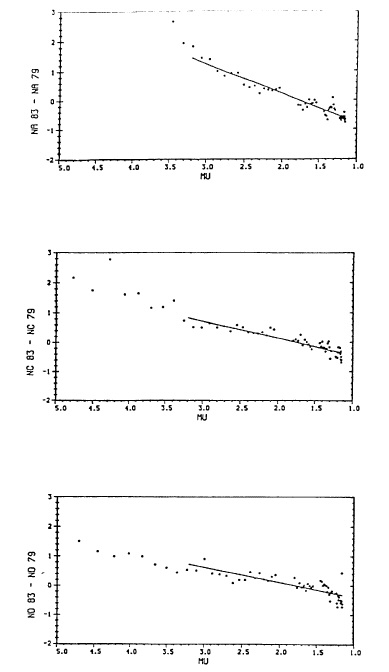
 FROM:                                                      N-TABLE
 G-TABLE                                                  INST.  79
 AUG 24, 1981                                          AUG 25, 1981
                                                       VERSION:  R1

                          NA TABLE

   R       0     1     2     3     4      5     6     7     8     9

   0   -31.4 -30.2 -29.1 -27.9 -26.7  -25.5 -24.3 -23.1 -22.0 -20.8
  10   -19.6 -18.4 -17.3 -16.2 -15.0  -13.9 -12.7 -11.6 -10.4  -9.2

  20    -8.0  -6.8  -5.6  -4.4  -3.2   -2.1   -.9    .3   1.4   2.6
  30     3.8   4.9   6.0   7.2   8.3    9.4  10.5  11.6  12.6  13.6
  40    14.6  15.6  16.6  17.6  18.5   19.5  20.4  21.4  22.4  23.3

  50    24.3  25.2  26.1  27.1  28.0   29.0  29.9  30.8  31.7  32.6
  60    33.5  34.5  35.4  36.3  37.2   38.1  39.0  39.9  40.8  41.7
  70    42.6  43.5  44.5  45.4  46.3   47.2  48.1  49.0  49.9  50.8
  80    51.7  52.6  53.6  54.5  55.5   56.4  57.3  58.3  59.2  60.2
  90    61.2  62.2  63.1  64.1  65.1   66.1  67.1  68.0  69.0  70.0

 100    71.0  72.0  73.0  74.1  75.1   76.1  77.1  78.1  79.1  80.1
 110    81.2  82.2  83.2  84.2  85.2   86.2  87.2  88.2  89.2  90.2
 120    91.3  92.3  93.3  94.3  95.3   96.3  97.4  98.4  99.4 100.4
 130   101.4 102.5 103.5 104.5 105.5  106.6 107.6 108.6 109.6 110.7
 140   111.7 112.7 113.7 114.7 115.7  116.8 117.8 118.8 119.8 120.8

 150   121.8 122.8 123.8 124.8 125.8  126.8 127.8 128.8 129.8 130.8
 160   131.8 132.8 133.9 134.9 135.9  136.9 137.9 138.9 139.9 140.9
 170   142.0 143.0 144.0 145.0 146.0  147.0 148.0 149.0 150.0 151.0
 180   152.0 153.0 154.0 155.0 156.0  157.0 158.0 159.0 160.0 161.0
 190   162.0 163.1 164.1 165.1 166.1  167.1 168.1 169.1 170.2 171.2

 200   172.2 173.2 174.3 175.3 176.3  177.3 178.4 179.4 180.4 181.4
 210   182.4 183.5 184.5 185.5 186.5  187.5 188.5 189.6 190.6 191.6
 220   192.6 193.6 194.7 195.7 196.7  197.7 198.8 199.8 200.8 201.9
 230   202.9 203.9 205.0 206.0 207.1  208.1 209.1 210.2 211.2 212.3
 240   213.3 214.4 215.4 216.5 217.6  218.6 219.7 220.7 221.8 222.9

 250   223.9 225.0 226.1 227.1 228.2  229.3 230.3 231.4 232.5 233.5
 260   234.6 235.6 236.6 237.7 238.7  239.7 240.7 241.8 242.8 243.8
 270   244.9 245.9 246.9 247.9 248.9  250.0 251.0 252.0 253.1 254.1
 280   255.2 256.2 257.3 258.4 259.5  260.6 261.7 262.8 263.9 265.0
 290   266.1 267.2 268.3 269.4

     TABLE GENERATED ON 92/05/26.
|
 FROM:                                                      N-TABLE
 G-TABLE                                                  INST.  79
 AUG 24, 1981                                          AUG 25, 1981
                                                       VERSION:  R1

                          NC TABLE

   R       0     1     2     3     4      5     6     7     8     9

  0    -31.1 -29.9 -28.8 -27.6 -26.5  -25.3 -24.2 -23.0 -21.9 -20.7
  10   -19.6 -18.4 -17.2 -16.0 -14.9  -13.7 -12.5 -11.3 -10.1  -9.0
  20    -7.8  -6.6  -5.5  -4.3  -3.2   -2.0   -.9    .2   1.3   2.4
  30     3.5   4.6   5.7   6.8   7.9    8.9  10.0  11.1  12.1  13.1
  40    14.1  15.1  16.1  17.1  18.1   19.1  20.1  21.0  22.0  23.0

  50    23.9  24.9  25.8  26.7  27.7   28.6  29.6  30.5  31.4  32.3
  60    33.2  34.1  35.0  35.9  36.8   37.7  38.7  39.6  40.5  41.4
  70    42.3  43.2  44.2  45.1  46.0   46.9  47.8  48.8  49.7  50.6
  80    51.6  52.5  53.4  54.4  55.3   56.3  57.2  58.2  59.1  60.1
  90    61.0  62.0  63.0  63.9  64.9   65.9  66.9  67.9  68.9  69.8

 100    70.8  71.8  72.8  73.8  74.8   75.8  76.8  77.8  78.8  79.8
 110    80.8  81.8  82.8  83.8  84.9   85.9  86.9  87.9  88.9  89.9
 120    90.9  91.9  92.9  93.9  94.9   95.9  96.9  98.0  99.0 100.0
 130   101.0 102.0 103.0 104.0 105.0  106.0 107.0 108.0 109.0 110.0
 140   111.0 112.0 113.0 114.0 115.0  116.0 117.0 117.9 118.9 119.9

 150   120.9 121.9 122.9 123.9 124.9  125.9 126.9 127.9 128.9 129.9
 160   130.9 131.9 132.9 133.8 134.8  135.8 136.8 137.8 138.8 139.7
 170   140.7 141.7 142.7 143.7 144.7  145.7 146.6 147.6 148.6 149.6
 180   150.6 151.6 152.6 153.6 154.6  155.6 156.6 157.6 158.6 159.6
 190   160.6 161.6 162.6 163.6 164.6  165.6 166.6 167.6 168.6 169.6

 200   170.6 171.6 172.6 173.6 174.6  175.6 176.6 177.6 178.6 179.6
 210   180.6 181.6 182.7 183.7 184.7  185.7 186.7 187.7 188.7 189.7
 220   190.7 191.7 192.7 193.7 194.7  195.7 196.7 197.7 198.7 199.7
 230   200.7 201.8 202.8 203.8 204.8  205.8 206.9 207.9 208.9 210.0
 240   211.0 212.0 213.1 214.1 215.2  216.2 217.3 218.3 219.4 220.4

 250   221.4 222.5 223.5 224.6 225.6  226.7 227.7 228.7 229.7 230.8
 260   231.8 232.8 233.9 234.9 235.9  236.9 237.9 239.0 240.0 241.0
 270   242.0 243.0 244.0 245.1 246.1  247.1 248.1 249.1 250.2 251.2
 280   252.2 253.3 254.3 255.4 256.4  257.5 258.6 259.7 260.8 261.9
 290   262.9 264.0 265.2 266.3 267.4  268.5 269.6

     TABLE GENERATED ON 92/05/26.
|
 FROM:                                                      N-TABLE
 G-TABLE                                                  INST.  79
 AUG 24, 1981                                          AUG 25, 1981
                                                       VERSION:  R1

                          ND TABLE

   R       0     1     2     3     4      5     6     7     8     9

   0   -33.4 -32.2 -31.1 -29.9 -28.8  -27.6 -26.5 -25.4 -24.2 -23.1
  10   -21.9 -20.8 -19.6 -18.5 -17.4  -16.2 -15.1 -14.0 -12.8 -11.7
  20   -10.5  -9.4  -8.3  -7.2  -6.1   -5.0  -3.8  -2.7  -1.6   -.5
  30      .6   1.6   2.7   3.8   4.9    5.9   7.0   8.1   9.1  10.1
  40    11.1  12.1  13.1  14.1  15.1   16.0  17.0  18.0  18.9  19.9

  50    20.9  21.8  22.7  23.7  24.6   25.6  26.5  27.4  28.4  29.3
  60    30.2  31.2  32.1  33.0  33.9   34.9  35.8  36.7  37.6  38.6
  70    39.5  40.4  41.3  42.3  43.2   44.1  45.1  46.0  46.9  47.9
  80    48.8  49.7  50.7  51.6  52.6   53.5  54.5  55.4  56.4  57.3
  90    58.3  59.3  60.2  61.2  62.2   63.1  64.1  65.1  66.1  67.1

 100    68.1  69.1  70.1  71.0  72.0   73.0  74.0  75.0  76.0  77.0
 110    78.0  79.0  80.0  81.0  82.0   83.0  84.0  85.0  86.0  87.0
 120    88.0  89.0  90.0  91.0  92.0   93.0  94.0  95.0  96.0  97.0
 130    98.0  99.0 100.0 101.0 102.0  103.0 104.0 105.0 106.0 107.0
 140   107.9 108.9 109.9 110.9 111.9  112.9 113.9 114.8 115.8 116.8

 150   117.8 118.8 119.8 120.7 121.7  122.7 123.7 124.6 125.6 126.6
 160   127.6 128.6 129.5 130.5 131.5  132.4 133.4 134.4 135.4 136.3
 170   137.3 138.3 139.3 140.2 141.2  142.2 143.2 144.1 145.1 146.1
 180   147.1 148.0 149.0 150.0 151.0  152.0 153.0 154.0 154.9 155.9
 190   156.9 157.9 158.9 159.8 160.8  161.8 162.8 163.8 164.8 165.8

 200   166.8 167.8 168.8 169.8 170.8  171.8 172.8 173.8 174.8 175.8
 210   176.8 177.8 178.8 179.8 180.8  181.8 182.8 183.8 184.8 185.8
 220   186.7 187.7 188.7 189.7 190.7  191.7 192.7 193.7 194.7 195.7
 230   196.7 197.7 198.7 199.7 200.7  201.7 202.7 203.8 204.8 205.8
 240   206.8 207.8 208.8 209.8 210.9  211.9 212.9 213.9 214.9 216.0

 250   217.0 218.0 219.0 220.1 221.1  222.1 223.2 224.2 225.2 226.2
 260   227.3 228.3 229.3 230.3 231.3  232.4 233.4 234.4 235.4 236.4
 270   237.4 238.4 239.4 240.4 241.4  242.4 243.4 244.4 245.4 246.4
 280   247.4 248.4 249.4 250.5 251.6  252.6 253.7 254.8 255.9 257.0
 290   258.1 259.2 260.3 261.5 262.6  263.7 264.8 265.9 267.1

     TABLE GENERATED ON 92/05/26.
|
  INST. NO:        79                           DATE:  Aug. 25, 1981R1

              REFERENCE STANDARD LAMP DATA
|
|||||||
Lamp No. |
Voltage |
Current |
RA |
RC |
RC' |
RD |
|
d.c. |
a.c. |
amps |
|||||
79Q1 79Q2 79Q3 UQ1 UQ2 UQ3 R12 R13 79C* 79D* |
24.0 24.0 24.0 24.0 24.0 24.0 24.0 24.0 |
100.0 100.0 |
      12.1
37.5

      12.6
38.0

      12.5
37.9

      13.9
39.3

      13.4
38.8

      12.6
38.0


37.7


38.0

      22.2
47.8

      22.0
48.6 |
      16.6
42.5

      17.1
43.0

      17.0
42.9

      18.2
44.1

      17.8
43.7

      16.8
42.7


42.8


42.8

      25.4
51.5

      25.6
51.7 |
      41.8
67.4

      41.3
68.9

      41.0
68.5

      39.0
66.3

      39.3
66.7

      40.8
68.3


67.9


67.9

      31.0
57.5


- |
      17.8
46.8

      18.3
47.3

      18.1
47.1

      19.5
48.6

      19.1
48.2

      18.2
47.2


46.8


47.3

      25.7
55.1

      25.8
55.2 |
|
NOTES: |
|||||||
|
 Data summary using Inst. 79 N tables dated     August 25, 1981:                         Calib Inst.  83 vs  79       June 19, 1985 AM

             1.15<MU<1.5     1.5<MU<2.0     2.0<MU<2.5     2.5<MU<3.2     3.2<MU<4.0     4.0<MU<5.0    1.15<MU<3.2

 XAD083*     .287 (.001)    .289 (.001)    .290 (.001)    .290 (.000)    .288 (.001)    .286 (.001)    .289 (.001) ATMO-CM
 XAD079*     .304 (.001)    .303 (.001)    .299 (.001)    .295 (.001)    .288 (.003)    .272 (.003)    .300 (.003) ATMO-CM
  DXAD079*         5.91           5.05           3.04           1.83           -.10          -4.98           3.95   PERCENT

 XCD083*     .283 (.004)    .286 (.003)    .286 (.001)    .285 (.001)    .284 (.001)    .285 (.000)    .285 (.001) ATMO-CM
 XCD079*     .302 (.006)    .310 (.003)    .310 (.002)    .305 (.003)    .296 (.002)    .291 (.001)    .307 (.003) ATMO-CM
  DXCD079*         6.49           8.35           8.28           6.99           4.32           1.85           7.53   PERCENT

 XA 083*     .295 (.001)    .297 (.001)    .297 (.001)    .296 (.000)    .294 (.001)    .291 (.001)    .296 (.001) ATMO-CM
 XA 079*     .305 (.001)    .305 (.001)    .303 (.001)    .300 (.001)    .295 (.003)    .281 (.003)    .303 (.002) ATMO-CM
  DXA 079*         3.20           2.69           2.03           1.45            .23          -3.36           2.34   PERCENT

 XC 083*     .301 (.001)    .302 (.001)    .300 (.001)    .298 (.001)    .296 (.000)    .295 (.000)    .301 (.002) ATMO-CM
 XC 079*     .303 (.002)    .307 (.001)    .311 (.000)    .309 (.001)    .305 (.001)    .301 (.001)    .308 (.003) ATMO-CM
  DXC 079*          .45           1.61           3.49           3.69           3.02           2.12           2.30   PERCENT

 XD 083*     .319 (.005)    .318 (.003)    .313 (.002)    .309 (.001)    .306 (.001)    .302 (.001)    .315 (.004) ATMO-CM
 XD 079*     .299 (.003)    .30O (.003)    .308 (.002)    .309 (.001)    .311 (.001)    .309 (.001)    .304 (.004) ATMO-CM
  DXD 079*        -6.14          -5.52          -1.65            .00           1.59           2.46          -3.36   PERCENT

 Corr. needed to Inst. 79 N values              mean     rad                                                          mean
             MU= 1.33   1.75   2.25   2.85   (1.15-2.5)                           MU= 1.33   1.75   2.25   2.85   (1.15-2.5)

 To NA ADD      -2.20  -2.47  -2.48  -2.13      -2.39  .230             To NAD ADD   -3.21  -3.44  -2.92  -2.02      -3.19

 To NC ADD       -.20  -1.01  -1.98  -2.69      -1.06  .152             To NCD ADD   -1.21  -1.98  -2.42  -2.58      -1.87

 To ND ADD       1.01    .97    .44   -.11        .80  .187

 Data summary using corrected Inst.  79 N Tables:   (using mean)

             1.15<MU<1.5     1.5<MU<2.0     2.0<MU<2.5     2.5<MU<3.2     3.2<MU<4.0     4.0<MU<5.0    1.15<MU<3.2

 XAD083      .287 (.001)    .289 (.001)    .290 (.001)    .290 (.000)    .288 (.001)    .286 (.001)    .289 (.001) ATMO-CM
 XAD079      .286 (.002)    .290 (.001)    .289 (.001)    .287 (.001)    .282 (.003)    .266 (.003)    .288 (.001) ATMO-CM
  DXAD079          -.17            .33           -.38           -.88          -2.32          -6.86           -.27   PERCENT

 XCD083      .283 (.004)    .286 (.003)    .286 (.001)    .285 (.001)    .284 (.001)    .285 (.000)    .285 (.001) ATMO-CM
 XCD079      .270 (.008)    .285 (.004)    .292 (.001)    .291 (.002)    .285 (.002)    .281 (.001)    .284 (.009) ATMO-CM
  DXCD079         -4.74           -.35           1.89           1.92            .31          -1.55           -.31   PERCENT

 XA 083      .295 (.001)    .297 (.001)    .297 (.001)    .296 (.000)    .294 (.001)    .291 (.001)    .296 (.001) ATMO-CM
 XA 079      .294 (.001)    .297 (.001)    .297 (.000)    .296 (.001)    .291 (.003)    .278 (.003)    .296 (.001) ATMO-CM
  DXA 079          -.32           -.05            .03           -.14          -1.07          -4.46           -.12   PERCENT

 XC 083      .301 (.001)    .302 (.001)    .300 (.001)    .298 (.001)    .296 (.000)    .295 (.000)    .301 (.002) ATMO-CM
 XC 079      .293 (.003)    .299 (.001)    .305 (.001)    .304 (.001)    .301 (.001)    .298 (.001)    .300 (.005) ATMO-CM
  DXC 079         -2.86          -1.03           1.56           2.17           1.82           1.09           -.05   PERCENT

 XD 083      .319 (.005)    .318 (.003)    .313 (.002)    .309 (.001)    .306 (.001)    .302 (.001)    .315 (.004) ATMO-CM
 XD 079      .316 (.004)    .314 (.002)    .318 (.001)    .317 (.001)    .317 (.001)    .315 (.001)    .316 (.002) ATMO-CM
  DXD 079          -.85          -1.37           1.45           2.49           3.57           4.17            .41   PERCENT

  Values in brackets are standard deviations.  NEW II BK O3 ABS. COEF. applied.
|
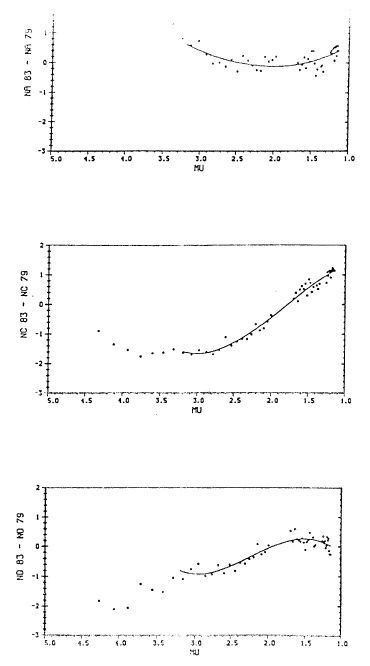
DOBSON INSTRUMENT 79 SAMPLE CALIBRATION DATA -
SEPTEMBER 10, 1975 AND AUGUST 14, 1981
(a) Unstable optical wedge.
(b) Observations are μ-dependent.
(c) Change in instrument optical characteristics occurred also due to cobalt filter corrosion.
|
                                                       INST. NO. 79
                                                 SEPTEMBER 09, 1975

                                  GA TABLE

   R       0     1     2     3     4      5     6     7     8     9
   0                                     .0   1.1   2.3   3.4   4.5
  10     5.7   6.9   8.0   9.2  10.4   11.6  12.8  14.0  15.2  16.4
  20    17.7  18.9  20.1  21.3  22.5   23.7  24.9  26.0  27.1  28.2
  30    29.4  30.5  31.6  32.7  33.8   34.9  36.0  37.0  38.1  39.1
  40    40.2  41.2  42.3  43.3  44.3   45.3  46.3  47.3  48.4  49.3

  50    50.3  51.3  52.3  53.3  54.2   55.2  56.1  57.0  57.9  58.9
  60    59.8  60.7  61.6  62.5  63.4   64.3  65.2  66.1  67.1  68.0
  70    68.9  69.9  70.8  71.7  72.6   73.6  74.5  75.5  76.4  77.4
  80    78.3  79.3  80.3  81.2  82.2   83.2  84.2  85.2  86.2  87.2
  90    88.2  89.2  90.2  91.2  92.2   93.2  94.2  95.3  96.3  97.3

 100    98.3  99.3 100.3 101.4 102.4  103.4 104.4 105.4 106.4 107.5
 110   108.5 109.5 110.5 111.5 112.6  113.6 114.6 115.6 116.7 117.7
 120   118.7 119.8 120.8 121.8 122.9  123.9 124.9 126.0 127.0 128.0
 130   129.0 130.1 131.1 132.1 133.1  134.1 135.1 136.2 137.2 138.2
 140   139.2 140.2 141.2 142.2 143.2  144.3 145.3 146.3 147.3 148.3

 150   149.4 150.4 151.4 152.4 153.5  154.5 155.5 156.5 157.5 158.6
 160   159.6 160.6 161.6 162.6 163.6  164.6 165.7 166.7 167.7 168.7
 170   169.7 170.7 171.7 172.7 173.8  174.8 175.8 176.8 177.9 178.9
 180   179.9 181.0 182.0 183.1 184.1  185.1 186.2 187.2 188.2 189.3
 190   190.3 191.4 192.4 193.4 194.5  195.5 196.6 197.6 198.6 199.7

 200   200.7 201.7 202.8 203.8 204.8  205.9 206.9 208.0 209.1 210.1
 210   211.2 212.2 213.3 214.3 215.4  216.4 217.5 218.5 219.5 220.6
 220   221.6 222.7 223.7 224.7 225.8  226.8 227.8 228.9 229.9 230.9
 230   231.9 233.0 234.0 235.0 236.1  237.1 238.2 239.2 240.2 241.3
 240   242.3 243.4 244.4 245.5 246.5  247.5 248.6 249.6 250.7 251.7

 250   252.8 253.8 254.9 255.9 256.9  258.0 259.0 260.0 261.0 262.1
 260   263.1 264.1 265.1 266.2 267.2  268.2 269.3 270.3 271.3 272.3
 270   273.4 274.4 275.4 276.5 277.5  278.6 279.6 280.6 281.7 282.7
 280   283.8 284.8 285.9 287.0 288.0  289.1 290.2 291.3 292.4 293.4
 290   294.5 295.6 296.8 297.9 299.1  300.2

 INPUT DATA:

   25.82  25.65  25.83  26.40  27.41  28.53  29.68  30.75
   31.52  32.00  32.24  32.17  31.70  31.18  30.69  30.28
   29.96  29.72  29.56  29.44  29.38  29.37  29.38  29.43
   29.48  29.53  29.57  29.59  29.60  29.59  29.54  29.47
   29.38  29.27  29.14  29.03  28.94  28.88  28.84  28.84
   28.88  28.93  28.98  29.01  29.00  28.98  28.97  29.01
   29.09  29.14  29.15  29.05  28.81  28.42  27.81
|
                                                       INST. NO. 79
                                                 SEPTEMBER 09, 1975

                                  GC TABLE

   R       0     1     2     3     4      5     6     7     8     9
   0                                     .0   1.1   2.3   3.4   4.5
  10     5.7   6.8   8.0   9.2  10.4   11.6  12.8  13.9  15.1  16.3
  20    17.5  18.7  19.8  21.0  22.1   23.3  24.4  25.5  26.6  27.7
  30    28.8  29.9  31.0  32.1  33.2   34.3  35.4  36.5  37.5  38.6
  40    39.7  40.7  41.8  42.8  43.8   44.8  45.8  46.8  47.8  48.8

  50    49.8  50.8  51.7  52.7  53.6   54.6  55.5  56.5  57.4  58.3
  60    59.2  60.2  61.1  62.0  63.0   63.9  64.8  65.8  66.7  67.7
  70    68.6  69.5  70.5  71.4  72.4   73.3  74.3  75.2  76.2  77.1
  80    78.1  79.1  80.0  81.0  82.0   83.0  84.0  84.9  85.9  86.9
  90    87.9  88.9  89.9  90.9  91.9   92.9  93.9  94.9  95.9  96.9

 100    97.9  98.9 100.0 101.0 102.0  103.0 104.0 105.0 106.0 107.0
 110   108.0 109.0 110.1 111.1 112.1  113.1 114.2 115.2 116.2 117.2
 120   118.2 119.3 120.3 121.3 122.3  123.3 124.3 125.4 126.4 127.4
 130   128.4 129.4 130.4 131.4 132.4  133.4 134.4 135.4 136.4 137.4
 140   138.4 139.4 140.4 141.4 142.4  143.5 144.5 145.5 146.5 147.5

 150   148.5 149.5 150.5 151.5 152.5  153.5 154.5 155.5 156.5 157.5
 160   158.5 159.5 160.5 161.5 162.5  163.5 164.5 165.5 166.6 167.6
 170   168.6 169.6 170.6 171.6 172.6  173.6 174.7 175.7 176.7 177.7
 180   178.8 179.8 180.8 181.8 182.9  183.9 184.9 185.9 186.9 188.0
 190   189.0 190.0 191.0 192.0 193.1  194.1 195.1 196.1 197.2 198.2

 200   199.2 200.3 201.3 202.3 203.4  204.4 205.4 206.5 207.5 208.6
 210   209.6 210.6 211.7 212.7 213.7  214.7 215.8 216.8 217.8 218.8
 220   219.9 220.9 221.9 222.9 223.9  225.0 226.0 227.0 228.0 229.0
 230   230.0 231.1 232.1 233.1 234.1  235.1 236.2 237.2 238.2 239.2
 240   240.3 241.3 242.3 243.3 244.4  245.4 246.4 247.4 248.5 249.5

 250   250.5 251.5 252.6 253.6 254.6  255.6 256.6 257.6 258.6 259.6
 260   260.6 261.6 262.6 263.7 264.7  265.7 266.7 267.7 268.7 269.8
 270   270.8 271.8 272.8 273.9 274.9  275.9 276.9 278.0 279.0 280.1
 280   281.1 282.2 283.2 284.3 285.4  286.4 287.5 288.5 269.6 290.7
 290   291.8 292.9 294.0 295.0

 INPUT DATA:

   26.37  26.14  26.31  26.89  27.77  28.73  29.69  30.62
   31.28  31.76  31.90  31.77  31.43  31.08  30.75  30.44
   30.17  29.93  29.77  29.68  29.66  29.67  29.72  29.78
   29.84  29.93  29.97  29.98  29.96  29.92  29.84  29.75
   29.66  29.56  29.46  29.37  29.30  29.25  29.23  29.24
   29.30  29.39  29.44  29.46  29.46  29.47  29.50  29.57
   29.62  29.61  29.54  29.32  29.08  28.66  28.02
|
                                                       INST. NO. 79
                                                 SEPTEMBER 09, 1975

                                  GD TABLE

   R       0     1     2     3     4      5     6     7     8     9
   0                                     .0   1.1   2.3   3.4   4.5
  10     5.6   6.8   8.0   9.1  10.3   11.5  12.6  13.8  14.9  16.1
  20    17.2  18.4  19.5  20.6  21.7   22.8  23.9  25.0  26.1  27.1
  30    28.2  29.3  30.4  31.4  32.5   33.6  34.7  35.7  36.8  37.8
  40    38.9  39.9  41.0  42.1  43.1   44.1  45.1  46.1  47.1  48.1

  50    49.1  50.0  51.0  52.0  52.9   53.9  54.8  55.8  56.7  57.6
  60    58.6  59.5  60.5  61.4  62.4   63.3  64.3  65.2  66.2  67.1
  70    68.1  69.0  70.0  70.9  71.9   72.9  73.8  74.8  75.8  76.7
  80    77.7  78.6  79.6  80.6  81.6   82.6  83.6  84.5  85.5  86.5
  90    87.5  88.5  89.5  90.5  91.5   92.5  93.5  94.5  95.5  96.5

 100    97.5  98.5  99.5 100.5 101.5  102.5 103.5 104.5 105.5 106.5
 110   107.5 108.5 109.6 110.6 111.6  112.6 113.6 114.6 115.6 116.6
 120   117.6 118.6 119.6 120.6 121.6  122.6 123.6 124.6 125.6 126.6
 130   127.6 128.6 129.6 130.6 131.6  132.6 133.6 134.6 135.6 136.5
 140   137.5 138.5 139.5 140.5 141.5  142.5 143.5 144.5 145.5 146.5

 150   147.5 148.5 149.5 150.5 151.5  152.5 153.5 154.5 155.5 156.4
 160   157.4 158.4 159.4 160.4 161.4  162.4 163.4 164.4 165.4 166.4
 170   167.4 168.4 169.4 170.4 171.4  172.4 173.4 174.4 175.4 176.4
 180   177.5 178.5 179.5 180.5 181.5  182.5 183.5 184.5 185.5 186.5
 190   187.5 188.6 189.6 190.6 191.6  192.6 193.6 194.6 195.6 196.6

 200   197.6 198.7 199.7 200.7 201.7  202.7 203.8 204.8 205.8 206.8
 210   207.9 208.9 209.9 210.9 211.9  213.0 214.0 215.0 216.0 217.0
 220   218.0 219.0 220.0 221.1 222.1  223.1 224.1 225.1 226.1 227.1
 230   228.1 229.1 230.1 231.1 232.1  233.1 234.1 235.1 236.1 237.2
 240   238.2 239.2 240.2 241.2 242.2  243.2 244.2 245.2 246.2 247.2

 250   248.2 249.2 250.2 251.2 252.2  253.2 254.2 255.2 256.2 257.2
 260   258.2 259.2 260.2 261.2 262.2  263.2 264.2 265.2 266.2 267.3
 270   268.3 269.3 270.3 271.3 272.3  273.3 274.3 275.4 276.4 277.4
 280   278.4 279.5 280.5 281.5 282.6  283.6 284.7 285.8 286.9 287.9
 290   289.0 290.1 291.3 292.4 293.5  294.6

 INPUT DATA:

   26.97  26.75  26.98  27.52  28.21  28.98  29.73  30.42
   31.03  31.42  31.60  31.43  31.16  30.90  30.66  30.43
   30.23  30.08  30.00  29.98  30.01  30.05  30.11  30.16
   30.22  30.25  30.27  30.29  30.27  30.22  30.17  30.08
   30.00  29.92  29.84  29.76  29.70  29.64  29.62  29.62
   29.65  29.73  29.81  29.86  29.91  29.95  29.97  29.99
   30.02  30.01  29.92  29.72  29.38  28.88  28.22
|
 Data summary using Inst. 79 G tables dated September  9, 1975:                         Calib Inst.  83 vs  79  September 10, 1975 AM

             1.15<MU<1.5     1.5<MU<2.0     2.0<MU<2.5     2.5<MU<3.2     3.2<MU<4.0     4.0<MU<5.0    1.15<MU<3.2

 XAD083*     .285 (.001)    .286 (.001)    .286 (.000)    .285 (.001)                                  .285 (.001) ATMO-CM
 XAD079*     .273 (.000)    .276 (.001)    .278 (.000)    .278 (.001)                                  .276 (.002) ATMO-CM
  DXAD079*        -4.21          -3.55          -2.69          -2.43                                        -3.22   PERCENT

 XCD083*     .292 (.001)    .291 (.001)    .288 (.001)    .284 (.001)                                  .289 (.003) ATMO-CM
 XCD079*     .242 (.001)    .246 (.006)    .258 (.001)    .259 (.002)                                  .251 (.007) ATMO-CM
  DXCD079*       -17.21         -15.36         -10.58          -8.49                                       -12.95   PERCENT

 XA 083*     .287 (.001)    .290 (.001)    .289 (.000)    .289 (.001)                                  .289 (.001) ATMO-CM
 XA 079*     .376 (.001)    .364 (.006)    .344 (.004)    .333 (.003)                                  .354 (.017) ATMO-CM
  DXA 079*        30.78          25.78          18.91          15.01                                        22.61   PERCENT

 XC 083*     .291 (.000)    .294 (.001)    .292 (.001)    .291 (.001)                                  .292 (.001) ATMO-CM
 XC 079*     .476 (.003)    .451 (.011)    .407 (.008)    .384 (.006)                                  .430 (.036) ATMO-CM
  DXC 079*        63.42          53.46          39.40          31.86                                        47.04   PERCENT

 XD 083*     .286 (.001)    .292 (.002)    .293 (.001)    .296 (.002)                                  .292 (.004) ATMO-CM
 XD 079*     .760 (.006)    .692 (.032)    .587 (.017)    .533 (.013)                                  .643 (.089) ATMO-CM
  DXD 079*       165.40         136.63         100.30          79.71                                       120.12   PERCENT

 Corr. needed to Inst. 79 G values              mean     rad                                                          mean
             MU= 1.33   1.75   2.25   2.85   (1.15-2.5)                           MU= 1.33   1.75   2.25   2.85   (1.15-2.5)

 To GA ADD     -23.41 -23.05 -22.63 -22.13     -23.03  .219             To GAD ADD    2.43   2.55   2.69   2.85       2.55

 To GC ADD     -22.39 -22.26 -22.10 -21.91     -22.25  .139             To GCD ADD    3.45   3.34   3.22   3.07       3.34

 To GD ADD     -25.84 -25.60 -25.32 -24.98     -25.59  .223

 Data summary using corrected Inst.  79 N Tables:   (using mean)

             1.15<MU<1.5     1.5<MU<2.0     2.0<MU<2.5     2.5<MU<3.2     3.2<MU<4.0     4.0<MU<5.0    1.15<MU<3.2

 XAD083      .285 (.001)    .286 (.001)    .286 (.000)    .285 (.001)                                  .285 (.001) ATMO-CM
 XAD079      .285 (.000)    .286 (.001)    .286 (.001)    .284 (.001)                                  .285 (.001) ATMO-CM
  DXAD079           .02            .02           -.03           -.29                                         -.07   PERCENT

 XCD083      .292 (.001)    .291 (.001)    .288 (.001)    .284 (.001)                                  .289 (.003) ATMO-CM
 XCD079      .292 (.002)    .290 (.003)    .290 (.002)    .286 (.002)                                  .289 (.002) ATMO-CM
  DXCD079          -.04           -.50            .60            .72                                          .19   PERCENT

 XA 083      .287 (.001)    .290 (.001)    .289 (.000)    .289 (.001)                                  .289 (.001) ATMO-CM
 XA 079      .288 (.001)    .290 (.000)    .288 (.000)    .288 (.001)                                  .288 (.001) ATMO-CM
  DXA 079           .34            .09           -.36           -.59                                         -.13   PERCENT

 XC 083      .291 (.000)    .294 (.001)    .292 (.001)    .291 (.001)                                  .292 (.001) ATMO-CM
 XC 079      .293 (.001)    .293 (.000)    .291 (.001)    .290 (.002)                                  .292 (.001) ATMO-CM
  DXC 079           .66           -.12           -.40           -.39                                         -.06   PERCENT

 XD 083      .286 (.001)    .292 (.002)    .293 (.001)    .296 (.002)                                  .292 (.004) ATMO-CM
 XD 079      .291 (.002)    .293 (.003)    .288 (.002)    .291 (.002)                                  .291 (.002) ATMO-CM
  DXD 079          1.55            .36          -1.61          -1.70                                         -.36   PERCENT

 Values in brackets are standard deviations. NEW II BK O3 ABS. COEF. applied.

 Cubic equations for N-function corrections to inst.  79 G-Tables
  A    -.2451477739E+02   .8355565381E+00    .0000000000E+00   .0000000000E+00
  C    -.2280700086E+02   .3147929774E+00    .0000000000E+00   .0000000000E+00
  D    -.2658217543E+02   .5610387537E+00    .0000000000E+00   .0000000000E+00
|
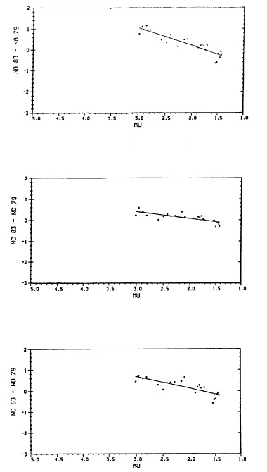
 FROM:                                                      N-TABLE
 G-TABLE                                                  INST.  79
 SEP  9, 1975                                          SEP 10, 1975
                                                       VERSION:  R1

                          NA TABLE

   R       0     1     2     3     4      5     6     7     8     9

   0   -28.7 -27.6 -26.4 -25.3 -24.2  -23.0 -21.9 -20.8 -19.6 -18.5
  10   -17.3 -16.2 -15.0 -13.8 -12.6  -11.5 -10.3  -9.0  -7.8  -6.6
  20    -5.4  -4.2  -3.0  -1.8   -.5     .7   1.8   3.0   4.1   5.2
  30     6.3   7.5   8.5   9.6  10.7   11.8  12.9  14.0  15.0  16.1
  40    17.1  18.2  19.2  20.2  21.3   22.3  23.3  24.3  25.3  26.3

  50    27.3  28.3  29.3  30.2  31.2   32.2  33.1  34.0  34.9  35.8
  60    36.7  37.7  38.6  39.5  40.4   41.3  42.2  43.1  44.0  45.0
  70    45.9  46.8  47.8  48.7  49.6   50.6  51.5  52.5  53.4  54.3
  80    55.3  56.3  57.2  58.2  59.2   60.2  61.1  62.1  63.1  64.1
  90    65.2  66.2  67.2  68.2  69.2   70.2  71.2  72.2  73.2  74.3

 100    75.3  76.3  77.3  78.3  79.3   80.4  81.4  82.4  83.4  84.4
 110    85.4  86.5  87.5  88.5  89.5   90.5  91.6  92.6  93.6  94.7
 120    95.7  96.7  97.8  98.8  99.8  100.9 101.9 102.9 103.9 105.0
 130   106.0 107.0 108.0 109.1 110.1  111.1 112.1 113.1 114.1 115.2
 140   116.2 117.2 118.2 119.2 120.2  121.2 122.2 123.3 124.3 125.3

 150   126.3 127.3 128.4 129.4 130.4  131.4 132.5 133.5 134.5 135.5
 160   136.5 137.6 138.6 139.6 140.6  141.6 142.6 143.6 144.7 145.7
 170   146.7 147.7 148.7 149.7 150.7  151.7 152.8 153.8 154.9 155.9
 180   156.9 158.0 159.0 160.0 161.1  162.1 163.1 164.2 165.2 166.3
 190   167.3 168.3 169.4 170.4 171.4  172.5 173.5 174.6 175.6 176.6

 200   177.7 178.7 179.7 180.8 181.8  182.9 183.9 185.0 186.0 187.1
 210   188.1 189.2 190.2 191.3 192.3  193.4 194.4 195.5 196.5 197.6
 220   198.6 199.6 200.7 201.7 202.7  203.8 204.8 205.8 206.9 207.9
 230   208.9 209.9 211.0 212.0 213.0  214.1 215.1 216.2 217.2 218.2
 240   219.3 220.3 221.4 222.4 223.5  224.5 225.6 226.6 227.7 228.7

 250   229.7 230.8 231.8 232.9 233.9  234.9 236.0 237.0 238.0 239.0
 260   240.1 241.1 242.1 243.1 244.2  245.2 246.2 247.3 248.3 249.3
 270   250.4 251.4 252.4 253.4 254.5  255.5 256.6 257.6 258.7 259.7
 280   260.8 261.8 262.9 263.9 265.0  266.1 267.2 268.2 269.3 270.4
 290   271.5 272.6 273.8 274.9 276.0  277.2
|
 FROM:                                                      N-TABLE
 G-TABLE                                                  INST.  79
 SEP  9, 1975                                          SEP 10, 1975
                                                       VERSION:  R1

                          NC TABLE

   R       0     1     2     3     4      5     6     7     8     9

   0   -27.9 -26.8 -25.7 -24.5 -23.4  -22.3 -21.1 -20.0 -18.8 -17.7
  10   -16.6 -15.4 -14.2 -13.0 -11.9  -10.7  -9.5  -8.3  -7.1  -5.9
  20    -4.7  -3.6  -2.4  -1.3   -.1    1.0   2.2   3.3   4.4   5.5
  30     6.6   7.7   8.8   9.9  11.0   12.1  13.2  14.3  15.3  16.4
  40    17.4  18.5  19.5  20.5  21.5   22.6  23.6  24.6  25.6  26.6

  50    27.5  28.5  29.5  30.4  31.4   32.3  33.3  34.2  35.1  36.1
  60    37.0  37.9  38.9  39.8  40.7   41.7  42.6  43.5  44.5  45.4
  70    46.4  47.3  48.2  49.2  50.1   51.1  52.0  53.0  53.9  54.9
  80    55.9  56.8  57.8  58.8  59.7   60.7  61.7  62.7  63.7  64.7
  90    65.7  66.7  67.7  68.7  69.7   70.7  71.7  72.7  73.7  74.7

 100    75.7  76.7  77.7  78.7  79.7   80.7  81.7  82.8  83.8  84.8
 110    85.8  86.8  87.8  88.8  89.9   90.9  91.9  92.9  93.9  95.0
 120    96.0  97.0  98.0  99.0 100.1  101.1 102.1 103.1 104.1 105.1
 130   106.1 107.1 108.1 109.2 110.2  111.2 112.2 113.2 114.2 115.2
 140   116.2 117.2 118.2 119.2 120.2  121.2 122.2 123.2 124.2 125.2

 150   126.2 127.3 128.3 129.3 130.3  131.3 132.3 133.3 134.3 135.3
 160   136.3 137.3 138.3 139.3 140.3  141.3 142.3 143.3 144.3 145.3
 170   146.3 147.3 148.3 149.4 150.4  151.4 152.4 153.4 154.5 155.5
 180   156.5 157.5 158.6 159.6 160.6  161.6 162.6 163.7 164.7 165.7
 190   166.7 167.7 168.8 169.8 170.8  171.8 172.9 173.9 174.9 175.9

 200   177.0 178.0 179.0 180.1 181.1  182.2 183.2 184.2 185.3 186.3
 210   187.3 188.4 189.4 190.4 191.5  192.5 193.5 194.5 195.6 196.6
 220   197.6 198.6 199.6 200.7 201.7  202.7 203.7 204.7 205.8 206.8
 230   207.8 208.8 209.8 210.8 211.9  212.9 213.9 214.9 216.0 217.0
 240   218.0 219.1 220.1 221.1 222.1  223.1 224.2 225.2 226.2 227.2

 250   228.3 229.3 230.3 231.3 232.3  233.3 234.4 235.4 236.4 237.4
 260   238.4 239.4 240.4 241.4 242.4  243.4 244.4 245.5 246.5 247.5
 270   248.5 249.6 250.6 251.6 252.6  253.7 254.7 255.7 256.8 257.8
 280   258.9 259.9 261.0 262.0 263.1  264.2 265.2 266.3 267.3 268.4
 290   269.5 270.6 271.7 272.8
|
FROM:                                                      N-TABLE
 G-TABLE                                                  INST.  79
 SEP  9, 1975                                          SEP 10, 1975
                                                       VERSION:  R1

                          ND TABLE

   R       0     1     2     3     4      5     6     7     8     9

   0   -31.2 -30.1 -29.0 -27.8 -26.7  -25.6 -24.5 -23.3 -22.2 -21.1
  10   -20.0 -18.8 -17.6 -16.5 -15.3  -14.1 -13.0 -11.8 -10.7  -9.5
  20    -8.4  -7.2  -6.1  -5.0  -3.9   -2.8  -1.7   -.6    .5   1.5
  30     2.6   3.7   4.8   5.9   6.9    8.0   9.1  10.1  11.2  12.3
  40    13.3  14.4  15.4  16.5  17.5   18.5  19.5  20.5  21.5  22.5

  50    23.5  24.5  25.4  26.4  27.3   28.3  29.2  30.2  31.1  32.1
  60    33.0  33.9  34.9  35.8  36.8   37.7  38.7  39.6  40.6  41.5
  70    42.5  43.4  44.4  45.4  46.3   47.3  48.2  49.2  50.2  51.1
  80    52.1  53.0  54.0  55.0  56.0   57.0  58.0  58.9  59.9  60.9
  90    61.9  62.9  63.9  64.9  65.9   66.9  67.9  68.9  69.9  70.9

 100    71.9  72.9  73.9  74.9  75.9   76.9  77.9  78.9  79.9  81.0
 110    82.0  83.0  84.0  85.0  86.0   87.0  88.0  89.0  90.0  91.0
 120    92.0  93.0  94.0  95.0  96.0   97.0  98.0  99.0 100.0 101.0
 130   102.0 103.0 104.0 105.0 106.0  107.0 108.0 109.0 110.0 111.0
 140   112.0 112.9 113.9 114.9 115.9  116.9 117.9 118.9 119.9 120.9

 150   121.9 122.9 123.9 124.9 125.9  126.9 127.9 128.9 129.9 130.9
 160   131.8 132.8 133.8 134.8 135.8  136.8 137.8 138.8 139.8 140.8
 170   141.8 142.8 143.6 144.8 145.8  146.8 147.8 148.8 149.8 150.8
 180   151.9 152.9 153.9 154.9 155.9  156.9 157.9 158.9 159.9 160.9
 190   162.0 163.0 164.0 165.0 166.0  167.0 168.0 169.0 170.0 171.0

 200   172.1 173.1 174.1 175.1 176.1  177.2 178.2 179.2 180.2 181.2
 210   182.3 183.3 184.3 185.3 186.3  187.4 188.4 189.4 190.4 191.4
 220   192.4 193.4 194.5 195.5 196.5  197.5 198.5 199.5 200.5 201.5
 230   202.5 203.5 204.5 205.5 206.5  207.5 208.5 209.6 210.6 211.6
 240   212.6 213.6 214.6 215.6 216.6  217.6 218.6 219.6 220.6 221.6

 250   222.6 223.6 224.6 225.6 226.6  227.6 228.6 229.6 230.6 231.6
 260   232.6 233.6 234.6 235.6 236.6  237.6 238.6 239.6 240.6 241.7
 270   242.7 243.7 244.7 245.7 246.7  247.7 248.7 249.8 250.8 251.8
 280   252.8 253.9 254.9 256.0 257.0  258.1 259.1 260.2 261.3 262.4
 290   263.4 264.5 265.7 266.8 267.9  269.1
|
  INST. NO:        79                           DATE:  Sept. 10, 1975

              REFERENCE STANDARD LAMP DATA
|
|||||||
Lamp No. |
Voltage |
Current |
RA |
RC |
RC' |
RD |
|
d.c. |
a.c. |
amps |
|||||
79C 79D W X Y Z |
100.0 100.0 100.0 100.0 100.0 100.0 |
      22.3
45.0

      23.3
46.0

      19.6
42.4


      20.1
42.9 |
      25.5
47.9

      26.2
48.6

      23.1
45.5


      23.3
45.7 |
      41.8
65.1

      42.3
65.7

      42.2
65.6


      43.9
67.4 |
      25.4
52.0

      26.0
52.6

      23.4
49.9


      23.3
49.8 |
||
NOTES: |
|||||||
|
 Data summary using Inst. 79 N tables dated September 10, 1975:                         Calib Inst.  65 vs  79     August 14, 1981 AM

             1.15<MU<1.5     1.5<MU<2.0     2.0<MU<2.5     2.5<MU<3.2     3.2<MU<4.0     4.0<MU<5.0    1.15<MU<3.2

 XAD065*     .299 (.003)    .298 (.001)    .299 (.000)    .298 (.000)    .297 (.001)    .294 (.000)    .299 (.000) ATMO-CM
 XAD079*     .315 (.004)    .309 (.001)    .305 (.002)                   .296 (.002)    .290 (.000)    .310 (.004) ATMO-CM
  DXAD079*         5.39           3.40           2.19                          -.25          -1.25           3.70   PERCENT

 XCD065*     .298 (.009)    .299 (.002)    .301 (.002)    .302 (.001)    .301 (.001)    .298 (.003)    .300 (.002) ATMO-CM
 XCD079*     .315 (.009)    .315 (.002)    .309 (.001)    .306 (.002)    .301 (.001)    .298 (.001)    .311 (.004) ATMO-CM
  DXCD079*         5.97           5.35           2.64           1.19           -.03            .10           3.78   PERCENT

 XA 065*     .306 (.002)    .307 (.001)    .307 (.000)    .306 (.001)    .304 (.001)    .302 (.000)    .306 (.001) ATMO-CM
 XA 079*     .320 (.003)    .316 (.001)    .313 (.001)                   .305 (.002)    .300 (.000)    .316 (.003) ATMO-CM
  DXA 079*         4.52           2.82           2.03                           .26           -.71           3.19   PERCENT

 XC 065*     .312 (.003)    .315 (.001)    .316 (.000)    .314 (.001)    .313 (.000)    .311 (.002)    .314 (.002) ATMO-CM
 XC 079*     .324 (.004)    .326 (.001)    .323 (.001)    .320 (.001)    .316 (.001)    .313 (.001)    .323 (.002) ATMO-CM
  DXC 079*         4.05           3.30           2.18           1.79            .96            .63           2.83   PERCENT

 XD 065*     .326 (.011)    .331 (.001)    .330 (.002)    .325 (.001)    .323 (.001)    .324 (.000)    .328 (.003) ATMO-CM
 XD 079*     .332 (.011)    .335 (.002)    .336 (.001)    .333 (.001)    .330 (.001)    .328 (.000)    .334 (.001) ATMO-CM
  DXD 079*         1.87           1.01           1.70           2.49           2.10           1.24           1.76   PERCENT

 Corr. needed to Inst. 79 N values              mean     rad                                                           mean
             MU= 1.33   1.75   2.25   2.85   (1.15-2.5)                            MU= 1.33   1.75   2.25   2.85   (1.15-2.5)

 To NA ADO      -3.06  -2.83  -2.55             -2.82   .211             To NAD ADD   -2.85  -2.46  -2.00             -2.44
 To NC ADD      -1.38  -1.37  -1.36  -1.34      -1.37   .152             To NCD ADO   -1.17  -1.00   -.81   -.57       -.99
 To NO ADD       -.22   -.37   -.55   -.77       -.38   .202

 Data summary using corrected Inst.  79 N Tables:   (using mean)

             1.15<MU<1.5     1.5<MU<2.0     2.0<MU<2.5     2.5<MU<3.2     3.2<MU<4.0     4.0<MU<5.0    1.15<MU<3.2

 XAD065      .299 (.003)    .298 (.001)    .299 (.000)    .298 (.000)    .297 (.001)    .294 (.000)    .299 (.000) ATMO-CM
 XAD079      .302 (.004)    .299 (.001)    .298 (.001)                   .291 (.002)    .286 (.000)    .299 (.002) ATMO-CM
  DXAD079           .83            .10           -.28                         -1.83          -2.64            .25   PERCENT

 XCDO65      .298 (.009)    .299 (.002)    .301 (.002)    .302 (.001)    .301 (.001)    .298(.003)     .300 (.002) ATMO-CM
 XCD079      .295 (.008)    .302 (.002)    .300 (.000)    .298 (.002)    .295 (.001)    .293(.001)     .300 (.002) ATMO-CM
  DXM079            .21           1.19           -.51          -1.36          -2.06         -1.63            -.12   PERCENT

 XA 065      .306 (.002)    .307 (.001)    .307 (.000)    .306 (.001)    .304 (.001)    .302(.000)     .306 (.001) ATMO-CM
 XA 079      .307 (.002)    .307 (.000)    .306 (.001)                   .301 (.002)    .296(.000)     .307 (.000) ATMO-CM
  DXA 079           .49           -.10           -.07                         -1.17         -1.95             .17   PERCENT

 XC 065      .312 (.003)    .315 (.001)    .316 (.000)    .314 (.001)    .313 (.000)    .311(.002)     .314 (.002) ATMO-CM
 XC 079      .311 (.003)    .316 (.001)    .316 (.001)    .314 (.001)    .311 (.000)    .309(.001)     .314 (.002) ATMO-CM
  DXC 079          -.18            .25           -.11           -.09           -.53          -.64            -.03   PERCENT

 XD 065      .326 (.011)    .331 (.001)    .330 (.002)    .325 (.001)    .323 (.001)    .324(.000)     .328 (.003) ATMO-CM
 XD 079      .324 (.011)    .329 (.002)    .331 (.001)    .330 (.001)    .327 (.001)    .325(.000)     .328 (.003) ATMO-CM
  DXD 079          -.62           -.77            .33           1.36           1.20           .47             .07   PERCENT

  Values in brackets are standard deviations.  NEW II BK O3 ABS. COEF. applied.

  Cubic equations for N-function corrections to inst.  79 G-Tables
   A    -.3795325355E+01   .5520981376E+00    .0000000000E+00   .0000000000E+00
   C    -.1419450791E+01   .2694022590E+01    .0000000000E+00   .0000000000E+00
   D     .2602520658E+00  -.3608938000E+00    .0000000000E+00   .0000000000E+00
|
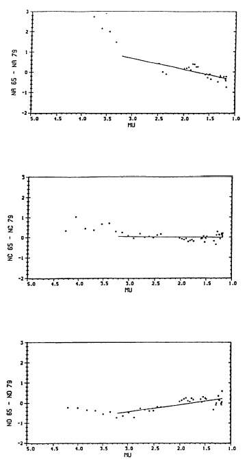
|
|
                                                       INST. NO. 79
                                                    AUGUST 24, 1981

                                  GA TABLE

   R       0     1     2     3     4      5     6     7     8     9

   0                                     .0   1.2   2.4   3.6   4.7
  10     5.9   7.1   8.2   9.3  10.5   11.6  12.8  13.9  15.1  16.3
  20    17.5  18.7  19.9  21.1  22.3   23.5  24.6  25.8  27.0  28.1
  30    29.3  30.4  31.5  32.7  33.8   34.9  36.0  37.1  38.1  39.1
  40    40.1  41.1  42.1  43.1  44.0   45.0  46.0  46.9  47.9  48.8

  50    49.8  50.7  51.6  52.6  53.5   54.5  55.4  56.3  57.2  58.1
  60    59.0  60.0  60.9  61.8  62.7   63.6  64.5  65.4  66.3  67.2
  70    68.1  69.1  70.0  70.9  71.8   72.7  73.6  74.5  75.4  76.3
  80    77.2  78.2  79.1  80.0  81.0   81.9  82.9  83.8  84.7  85.7
  90    86.7  87.7  88.6  89.6  90.6   91.6  92.6  93.6  94.5  95.5

 100    96.5  97.5  98.6  99.6 100.6  101.6 102.6 103.6 104.6 105.6
 110   106.7 107.7 108.7 109.7 110.7  111.7 112.7 113.7 114.7 115.8
 120   116.8 117.8 118.8 119.8 120.8  121.8 122.9 123.9 124.9 125.9
 130   127.0 128.0 129.0 130.0 131.1  132.1 133.1 134.1 135.2 136.2
 140   137.2 138.2 139.2 140.2 141.3  142.3 143.3 144.3 145.3 146.3

 150   147.3 148.3 149.3 150.3 151.3  152.3 153.3 154.3 155.3 156.3
 160   157.3 158.4 159.4 160.4 161.4  162.4 163.4 164.4 165.4 166.5
 170   167.5 168.5 169.5 170.5 171.5  172.5 173.5 174.5 175.5 176.5
 150   177.5 178.5 179.5 180.5 181.5  182.5 183.5 184.5 185.5 186.5
 190   187.6 188.6 189.6 190.6 191.6  192.6 193.6 194.7 195.7 196.7

 200   197.7 198.8 199.8 200.8 201.8  202.8 203.9 204.9 205.9 206.9
 210   207.9 209.0 210.0 211.0 212.0  213.0 214.0 215.1 216.1 217.1
 220   218.1 219.1 220.2 221.2 222.2  223.2 224.3 225.3 226.3 227.4
 230   228.4 229.5 230.5 231.5 232.6  233.6 234.6 235.7 236.8 237.8
 240   238.9 239.9 241.0 242.0 243.1  244.1 245.2 246.3 247.3 248.4

 250   249.5 250.5 251.6 252.7 253.7  254.8 255.8 256.9 258.0 259.0
 260   260.1 261.1 262.1 263.2 264.2  265.2 266.2 267.3 268.3 269.3
 270   270.4 271.4 272.4 273.4 274.5  275.5 276.5 277.5 278.6 279.6
 280   280.7 281.7 282.8 283.9 285.0  286.1 287.2 288.3 289.4 290.5
 290   291.6 292.7 293.8 294.9


 INPUT DATA:

   25.82  25.71  25.98  26.53  27.70  29.04  30.38  31.67
   32.36  32.69  32.88  32.83  32.55  32.18  31.71  31.20
   30.65  30.26  30.00  29.82  29.69  29.62  29.57  29.55
   29.56  29.62  29.71  29.78  29.84  29.88  29.89  29.91
   29.90  29.89  29.85  29.77  29.67  29.59  29.55  29.50
   29.44  29.37  29.25  29.06  28.84  28.64  28.50  28.52
   28.62  28.80  28.96  28.96  28.76  28.34  27.88
|
                                                       INST. NO. 79
                                                    AUGUST 24, 1981

                                  GC TABLE

   R       0     1     2     3     4      5     6     7     8     9

   0                                     .0   1.1   2.3   3.4   4.6
  10     5.7   6.9   8.1   9.3  10.5   11.7  12.8  14.0  15.2  16.4
  20    17.6  18.7  19.9  21.0  22.2   23.3  24.4  25.5  26.7  27.8
  30    28.9  30.0  31.0  32.1  33.2   34.3  35.4  36.4  37.4  38.4
  40    39.4  40.5  41.5  42.5  43.4   44.4  45.4  46.4  47.3  48.3

  50    49.3  50.2  51.1  52.1  53.0   54.0  54.9  55.8  56.7  57.6
  60    58.5  59.4  60.4  61.3  62.2   63.1  64.0  64.9  65.8  66.7
  70    67.6  68.6  69.5  70.4  71.3   72.3  73.2  74.1  75.0  76.0
  80    76.9  77.8  78.8  79.7  80.7   81.6  82.6  83.5  84.4  85.4
  90    86.4  87.3  88.3  89.3  90.2   91.2  92.2  93.2  94.2  95.2

 100    96.2  97.2  98.2  99.2 100.2  101.2 102.2 103.2 104.2 105.2
 110   106.2 107.2 108.2 109.2 110.2  111.2 112.2 113.2 114.2 115.2
 120   116.2 117.2 118.3 119.3 120.3  121.3 122.3 123.3 124.3 125.3
 130   126.3 127.3 128.3 129.3 130.3  131.3 132.3 133.3 134.3 135.3
 140   136.3 137.3 138.3 139.3 140.3  141.3 142.3 143.3 144.3 145.3

 150   146.3 147.3 148.3 149.3 150.3  151.3 152.2 153.2 154.2 155.2
 160   156.2 157.2 158.2 159.2 160.2  161.2 162.1 163.1 164.1 165.1
 170   166.1 167.1 168.0 169.0 170.0  171.0 172.0 173.0 174.0 175.0
 180   176.0 176.9 177.9 178.9 179.9  180.9 181.9 182.9 183.9 184.9
 190   185.9 186.9 187.9 188.9 189.9  190.9 191.9 192.9 193.9 194.9

 200   195.9 196.9 197.9 198.9 199.9  200.9 201.9 202.9 204.0 205.0
 210   206.0 207.0 208.0 209.0 210.0  211.0 212.0 213.0 214.0 215.0
 220   216.0 217.0 218.0 219.0 220.0  221.0 222.0 223.1 224.1 225.1
 230   226.1 227.1 228.1 229.1 230.2  231.2 232.2 233.2 234.3 235.3
 240   236.3 237.4 238.4 239.5 240.5  241.6 242.6 243.7 244.7 245.7

 250   246.8 247.8 248.9 249.9 250.9  252.0 253.0 254.1 255.1 256.1
 260   257.1 258.2 259.2 260.2 261.2  262.3 263.3 264.3 265.3 266.3
 270   267.3 268.4 269.4 270.4 271.4  272.4 273.5 274.5 275.5 276.5
 280   277.6 278.6 279.7 280.7 281.8  282.8 283.9 285.0 286.1 287.2
 290   288.3 289.4 290.5 291.6 292.7  293.9 295.0


 INPUT DATA:

   26.28  26.12  26.44  27.27  28.33  29.40  30.47  31.54
   32.12  32.48  32.68  32.62  32.38  31.98  31.59  31.20
   30.81  30.49  30.22  30.04  29.94  29.93  29.94  29.99
   30.07  30.13  30.21  30.29  30.37  30.42  30.43  30.43
   30.42  30.36  30.28  30.17  30.07  30.01  29.97  29.95
   29.93  29.87  29.76  29.58  29.38  29.18  29.03  29.01
   29.10  29.26  29.36  29.32  29.10  28.67  28.23
|
                                                        INST. NO. 79
                                                     AUGUST 24, 1981

                                   GD TABLE

    R       0     1     2     3     4      5     6     7     8     9

   0                                      .0   1.1   2.3   3.4   4.6
  10      5.7   6.9   8.0   9.1  10.3   11.4  12.6  13.7  14.8  16.0
  20     17.1  18.2  19.4  20.5  21.6   22.7  23.8  24.9  26.0  27.1
  30     28.2  29.3  30.4  31.5  32.5   33.6  34.7  35.7  36.8  37.8
  40     38.8  39.8  40.8  41.8  42.7   43.7  44.7  45.6  46.6  47.6

  50     48.5  49.5  50.4  51.3  52.3   53.2  54.2  55.1  56.0  56.9
  60     57.9  58.8  59.7  60.7  61.6   62.5  63.4  64.4  65.3  66.2
  70     67.1  68.1  69.0  69.9  70.8   71.8  72.7  73.6  74.6  75.5
  80     76.4  77.4  78.3  79.3  80.2   81.2  82.1  83.1  84.0  85.0
  90     85.9  86.9  87.9  88.8  89.8   90.8  91.8  92.8  93.8  94.7

 100     95.7  96.7  97.7  98.7  99.7  100.7 101.7 102.7 103.7 104.7
 110    105.7 106.6 107.6 108.6 109.6  110.6 111.6 112.6 113.6 114.6
 120    115.6 116.6 117.7 118.7 119.7  120.7 121.7 122.7 123.7 124.7
 130    125.7 126.7 127.7 128.7 129.7  130.7 131.6 132.6 133.6 134.6
 140    135.6 136.6 137.6 138.5 139.5  140.5 141.5 142.5 143.5 144.5

 150    145.4 146.4 147.4 148.4 149.4  150.3 151.3 152.3 153.3 154.3
 160    155.2 156.2 157.2 158.2 159.1  160.1 161.1 162.0 163.0 164.0
 170    165.0 165.9 166.9 167.9 168.8  169.8 170.8 171.8 172.8 173.7
 180    174.7 175.7 176.7 177.7 178.6  179.6 180.6 181.6 182.6 183.6
 190    184.5 185.5 186.5 187.5 188.5  189.5 190.5 191.5 192.4 193.4

 200    194.4 195.4 196.4 197.4 198.4  199.4 200.4 201.4 202.4 203.4
 210    204.4 205.4 206.4 207.4 208.4  209.4 210.4 211.4 212.4 213.4
 220    214.4 215.4 216.4 217.4 218.4  219.4 220.4 221.4 222.4 223.4
 230    224.4 225.4 226.4 227.4 228.4  229.4 230.4 231.4 232.4 233.4
 240    234.4 235.5 236.5 237.5 238.5  239.5 240.5 241.6 242.6 243.6

 250    244.6 245.7 246.7 247.7 248.7  249.8 250.8 251.8 252.9 253.9
 260    254.9 255.9 257.0 258.0 259.0  260.0 261.0 262.0 263.0 264.1
 270    265.1 266.1 267.0 268.0 269.0  270.0 271.0 272.0 273.0 274.0
 280    275.0 276.1 277.1 278.1 279.2  280.3 281.4 282.4 283.5 284.6
 290    285.8 286.9 288.0 289.1 290.2  291.3 292.5 293.6 294.7


 INPUT DATA:

   26.79  26.73  27.07  27.75  28.64  29.56  30.47  31.37
   31.97  32.20  32.33  32.29  32.15  31.85  31.52  31.20
   30.89  30.61  30.38  30.22  30.13  30.12  30.16  30.22
   30.31  30.43  30.58  30.68  30.77  30.82  30.85  30.83
   30.82  30.74  30.63  30.50  30.38  30.30  30.24  30.21
   30.18  30.15  30.10  30.02  29.88  29.71  29.55  29.47
   29.46  29.62  29.77  29.68  29.38  28.90  28.42
|
 Data summary using Inst. 79 G tables dated    August 24, 1981:                          Calib Inst.  65 vs  79     August 14, 1981 AM

             1.15<MU<1.5     1.5<MU<2.0     2.0<MU<2.5     2.5<MU<3.2     3.2<MU<4.0     4.0<MU<5.0    1.15<MU<3.2

 XAD065*     .299 (.003)    .298 (.001)    .299 (.000)    .298 (.000)    .297 (.001)    .294 (.000)    .299 (.000) ATMO-CM
 XAD079*     .308 (.004)    .304 (.001)    .301 (.002)                   .293 (.002)    .288 (.000)    .304 (.003) ATMO-CM
  DXAD079*         3.10           1.78            .85                         -1.13          -1.83           1.94   PERCENT

 XCD065*     .298 (.009)    .299 (.002)    .301 (.002)    .302 (.001)    .301 (.001)    .298 (.003)    .300 (.002) ATMO-CM
 XCD079*     .306 (.008)    .305 (.002)    .302 (.000)    .301 (.001)    .298 (.001)    .293 (.002)    .304 (.002) ATMO-CM
  DXCD079*         2.88           1.93            .27           -.25          -1.13          -1.44           1.20   PERCENT

 XA 065*     .306 (.002)    .307 (.001)    .307 (.000)    .306 (.001)    .304 (.001)    .302 (.000)    .306 (.001) ATMO-CM
 XA 079*     .314 (.003)    .311 (.001)    .308 (.001)                   .301 (.001)    .297 (.000)    .311 (.002) ATMO-CM
  DXA 079*         2.73           1.30            .46                         -1.03          -1.72           1.56   PERCENT

 XC 065*     .312 (.003)    .315 (.001)    .316 (.000)    .314 (.001)    .313 (.000)    .311 (.002)    .314 (.002) ATMO-CM
 XC 079*     .319 (.004)    .318 (.001)    .316 (.001)    .314 (.001)    .310 (.001)    .307 (.001)    .317 (.002) ATMO-CM
  DXC 079*         2.41            .98           -.08           -.28           -.93          -1.39            .75   PERCENT

 XD 065*     .326 (.011)    .331 (.001)    .330 (.002)    .325 (.001)    .323 (.001)    .324 (.000)    .328 (.003) ATMO-CM
 XD 079*     .331 (.011)    .331 (.002)    .328 (.002)    .324 (.001)    .321 (.001)    .320 (.000)    .329 (.003) ATMO-CM
  DXD 079*         1.76           -.16           -.48           -.33            .71          -1.35            .19   PERCENT

 Corr. needed to Inst. 79 G values              mean     rad                                                           mean
             MU= 1.33   1.75   2.25   2.85   (1.15-2.5)                            MU= 1.33   1.75   2.25   2.85   (1.15- 2.5)

 To GA ADD      -1.81  -1.29   -.69             -1.26  .166              To GAD ADD   -1.63  -1.22   -.74             -1.20

 To GC ADD       -.71   -.43   -.10    .29       -.41  .129              To GCD ADD    -.53   -.36   -.16    .08       -.35

 To GD ADD       -.18   -.07    .06    .21       -.07  .190

 Data summary using corrected Inst.  79 N Tables:   (using mean)

             1.15<MU<1.5     1.5<MU<2.0     2.0<MU<2.5     2.5<MU<3.2     3.2<MU<4.0     4.0<MU<5.0    1.15<MU<3.2

 XAD065      .299 (.003)    .298 (.001)    .299 (.000)    .298 (.000)    .297 (.001)    .294 (.000)    .299 (.000) ATMO-CM
 XAD079      .302 (.004)    .299 (.001)    .298 (.001)                   .291 (.002)    .286 (.000)    .299 (.002) ATMO-CM
  DXAD079           .86            .15           -.36                         -1.90          -2.52            .25   PERCENT

 XCD065      .298 (.009)    .299 (.002)    .301 (.002)    .302 (.001)    .301 (.001)    .298 (.003)    .300 (.002) ATMO-CM
 XCD079      .300 (.008)    .300 (.002)    .299 (.000)    .299 (.001)    .296 (.001)    .292 (.002)    .299 (.001) ATMO-CM
  DXCD079           .85           -.46           -.84          -1.15          -1.84          -2.05           -.17   PERCENT

 XA 065      .306 (.002)    .307 (.001)    .307 (.000)    .306 (.001)    .304 (.001)    .302 (.000)    .306 (.001) ATMO-CM
 XA 079      .309 (.002)    .307 (.000)    .305 (.001)                   .299 (.001)    .295 (.000)    .307 (.001) ATMO-CM
  DXA 079           .92           -.00           -.48                         -1.67          -2.27            .21   PERCENT

 XC 065      .312 (.003)    .315 (.001)    .316 (.000)    .314 (.001)    .313 (.000)    .311 (.002)    .314 (.002) ATMO-CM
 XC 079      .315 (.003)    .316 (.001)    .314 (.001)    .312 (.001)    .309 (.001)    .306 (.001)    .314 (.001) ATMO-CM
  DXC 079          1.13            .06           -.78           -.85          -1.38          -1.77           -.11   PERCENT

 XD 065      .326 (.011)    .331 (.001)    .330 (.002)    .325 (.001)    .323 (.001)    .324 (.000)    .328 (.003) ATMO-CM
 XD 079      .330 (.011)    .330 (.002)    .328 (.002)    .324 (.001)    .320 (.001)    .319 (.000)    .328 (.003) ATMO-CM
  DXD 079          1.33           -.47           -.71           -.52           -.86          -1.48           -.09   PERCENT

 Values in brackets are standard deviations.  NEW II BK O3 ABS. COEF. applied.

  Cubic equations for N-function corrections to inst.  79 G-Tables
   A    -.3403727558E+01   .1206449254E+01    .0000000000E+00   .0000000000E+00
   C    -.1580171279E+01   .6565992229E+00    .0000000000E+00   .0000000000E+00
   D    -.5165673688E+00   .2542950991E+00    .0000000000E+00   .0000000000E+00
|