|
Overview
Results
Resources
|
|
Documentation - CT2011_oi
|
|
|
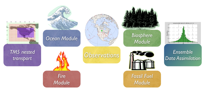
To learn more about a CarbonTracker component, click on one of the above images.
Or download the full PDF version for convenience.
|
|
1. Introduction
Human beings first influenced the carbon cycle through land-use
change. Early humans used fire to control animals and later cleared
forest for agriculture. Over the last two centuries, following the
industrial and technical revolutions and the world population
increase, fossil fuel combustion has become the largest anthropogenic
source of CO2. Coal, oil and natural gas
combustion are the most common energy sources in both developed
and developing countries. Various sectors of the economy rely on
fossil fuel combustion: power generation, transportation,
residential/commercial building heating, and industrial processes.
In 2008, the world emissions of CO2 from
fossil fuel burning, cement manufacturing, and flaring reached
8.7 PgC yr-1 (one
PgC=1015 grams of carbon) [Boden et al.,
2011] and we estimate the global total emissions for 2009 and 2010 to
be 8.6 PgC yr-1 and
9.1 PgC yr-1 respectively [Boden et
al., 2011]. The 2010 figure represents a 47% increase over 1990 emissions. The
North American (U.S.A, Canada, and Mexico) input of
CO2 to the atmosphere from fossil fuel
burning was 1.8 PgC in 2008, representing 21% of the global
total. North American emissions have remained nearly constant since
2000. On the other hand, emissions from developing economies such as
the People's Republic of China have been increasing. The Department
of Energy's 2011 International Energy Outlook has projected that the
global total source will reach
9.1 PgC yr-1 in 2015 and
11.1 PgC yr-1 in 2030
[DOE].
Despite the recent economic slowdown, which affected developing countries starting in 2008, fossil
fuel emissions in many parts of the world continue to increase.
In many flux estimation systems, including CarbonTracker, fossil fuel
CO2 emissions are specified. These imposed
emissions are not optimized in the estimation framework. Thus, fossil
fuel CO2 emissions must be prescribed
accurately in order to yield robust flux estimates for the land
biosphere and oceans. Fossil fuel emissions estimates we use are
available on an annually-integrated global and national basis, and
this information needs to be gridded before being incorporated into
CarbonTracker. The major uncertainty in this process is distributing
the national-annual emissions spatially across a nation and temporally
into monthly contributions. In CT2011, two different fossil fuel
CO2 emissions datasets were used to help
assess the uncertainty in this mapping process. The legacy
CarconTracker fossil fuel product ("Miller") has this year been
augmented with the "ODIAC" [Oda and Maksyutov, 2011] emissions
product. These two datasets share the same global and national
emissions for each year, but differ in how those emissions are
distributed spatially and temporally.
|
|
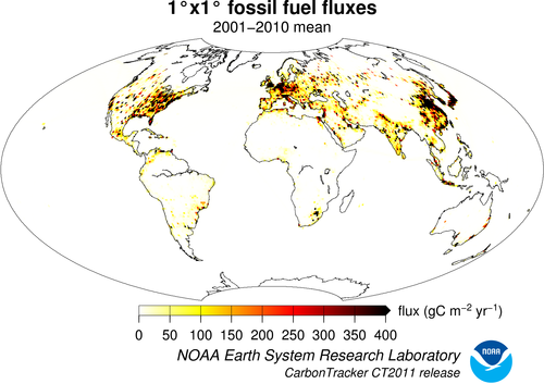
Figure 1. Spatial distribution of fossil fuel emissions. This is a spatial average of the Miller and ODIAC emissions inventories.
|
2. The "Miller" emissions dataset
- Totals
The Miller fossil fuel emission inventory is derived from independent
global total and spatially-resolved inventories. Annual global total
fossil fuel CO2 emissions are from the Carbon
Dioxide Information and Analysis Center (CDIAC) [Boden et al. 2011]
which extend through 2008. In order to extrapolate these fluxes to
2009 and 2010, we extrapolate using the percentage increase or
decrease for each fuel type (solid, liquid, and gas) in each country
from the 2011 BP Statistical Review of World Energy for 2009 and 2010.
- Spatial Distribution
Miller fossil-fuel
CO2 fluxes are spatially distributed in two
steps: First, the coarse-scale flux distribution country totals from
Boden et al. [2011] are mapped onto
a 1°x1° grid. Next, we distribute the
country totals within countries according to the spatial patterns from
the EDGAR v4.0 inventories [European Commission, 2009], which are
annual estimates also at 1°x1° resolution. The CDIAC
country-by-country totals, however, only sum to about 95% of the
global total. We ascribe the difference to land regions according to
the relative pattern of emissions over the globe.
- Temporal Distribution
For North America between 30 and 60°N, the Miller system imposes a
normalized, annually-invariant, seasonal cycle on emissions. This
annual cycle is derived by extracting the first and second harmonics
[Thoning et al, 1989] from the Blasing et al. [2005] analysis for the
United States. The Blasing analysis has ~10% higher emissions in
winter than in summer.
For Eurasia, a set of seasonal emissions factors from EDGAR,
distributed by emissions sector, is used to define fossil fuel
seasonality. As in North America, this seasonality is imposed only
from 30-60°N. The Eurasian seasonal amplitude is about 25%,
significantly larger than that in North America, owing to the absence
of a secondary summertime maximum due to air conditioning.
See Box 1 for the resulting time series of fossil fuel emissions. In order to
avoid discontinuities in the fossil fuel emissions
between consecutive years, a spline curve that conserves annual totals
[Rasmussen 1991] is fit to seasonal emissions in each 1°x1°
grid cell.
3. The "ODIAC" emissions dataset
- Totals
The ODIAC fossil fuel emission inventory [Oda and Maksyutov, 2011] is
also derived from independent global and country emission estimates
from CDIAC, but from the previous year’s estimates [Boden et
al. 2010]. Annual country total fossil fuel
CO2 emissions from CDIAC which extend through
2007, were extrapolated to 2008, 2009 and 2010 using the BP
Statistical Review of World Energy. The difference between the CDIAC
global total and country-by-country totals were ascribed to the entire
emissions fields. The same adjustment was done for 2009 and 2010 using
preliminary 2009 and 2010 estimates by CDIAC.
- Spatial Distribution
ODIAC emissions are spatially distributed using many available “proxy
data” that explain spatial extent of emissions according to emission
types (emissions over land, gas flaring, aviation and marine
bunker). Emissions over land were distributed in two steps: First,
emissions attributable to power plants were mapped using geographical
locations (latitude and longitude) provided by the global power plant
data CARMA. Next, the remaining land emissions (i.e. land total minus
power plant emissions) were distributed using nightlight imagery
collected by U.S. Air Force Defense Meteorological Satellite Project
(DMSP) satellites. Emissions from gas flaring were also mapped using
nightlight imagery. Emissions from aviation were mapped using flight
tracks adopted from UK AERO2k air emission inventory. It should be
noted that currently, air traffic emissions are emitted at ground
level within CarbonTracker. Emissions from marine bunker fuels are
placed entirely in the ocean basins along shipping routes according to
patterns from the EDGAR database.
- Temporal Distribution
The CDIAC estimates used for mapping emissions in ODIAC only describe
how much CO2 was emitted in a given year. To
present seasonal changes in emissions, we used the CDIAC 1°x1°
monthly fossil fuel emission inventory [Andres et al. 2011]. The CDIAC
monthly data utilizes the top 20 emitting countries' fuel (coal, oil
and gas) consumption statistics available to estimate seasonal change
in emissions. Monthly emission numbers at each pixel were divided by
annual total and then a fraction to annual total was obtained. Monthly
emissions in the ODIAC inventory were derived by multiplying this
fraction by the emission in each grid cell.
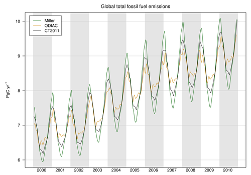
Box 1. Comparison of the Miller and ODIAC global fossil fuel emissions estimates
|
|
Time series of global fossil fuel emissions. The Miller (green) and ODIAC (tan) estimates are each used by half of the eight inversions in the CT2011 suite, so the CT2011 (black) inventory is effectively an average of Miller and ODIAC. Note that fossil fuel emissions are not optimized in CarbonTracker.
|
|
|
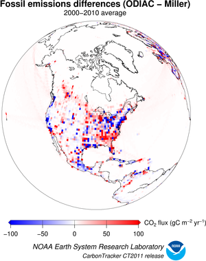
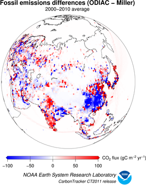
Spatial differences in long-term mean fossil fuel
emissions. between the two priors Note that both the Miller
and ODIAC emissions inventories use the same country totals,
but have different models for spatial distribution of that
flux within countries.
|
Uncertainties
The uncertainty attached to the global total source is of order 5% (2
sigma) until 2007 [Marland, 2008], but the uncertainties for individual
regions of the world, and for sub-annual time periods are likely to be
larger. Additional uncertainties are further introduced when the
emissions are distributed in space and time. In the Miller dataset,
the overall Eurasian seasonality is uncertain, but most likely a
better representation than assuming no emission seasonality at
all. Similarly, the use of the CDIAC monthly emission dataset for modeling
seasonality introduces additional uncertainty in ODIAC. The additional
uncertainty for the global total in the monthly CDIAC emission, which
is solely due to the method for estimating seasonality, is reported as
6.4% [Andres et al. 2011]. As mentioned earlier, fossil fuel emissions
are not optimized in the current CarbonTracker system, similar to many
similar global carbon data analysis systems.
Spatial and temporal atmospheric CO2
gradients arise from terrestrial biosphere and fossil-fuel sources.
These gradients, which are interpreted by CarbonTracker, are difficult
to attribute to one or the other cause. This is because the
biospheric and anthropogenic sources are often co-located, especially
in the temperate Northern Hemisphere.
Given that surface CO2 flux due to biospheric
activity and oceanic exchange is much more uncertain compared to
fossil fuel emissions, CarbonTracker, like most current carbon dioxide
data assimilation systems, does not optimize fossil fuel emissions.
The contribution of CO2 from fossil fuel
burning to observed CO2 mole fractions is
considered known. However, for the first time in CarbonTracker, an
effort is made to account for some aspects of fossil fuel uncertainty
by using two different fossil fuel estimates as detailed above. From
a technical point of view, extra land biosphere prior flux uncertainty
is included in the system to represent the random errors in fossil
fuel emissions. Eventually, fossil fuel emissions could be optimized within
CarbonTracker, especially with the addition
of 14CO2
observations as constraints.
3. Further Reading
- CDIAC (Boden et al.) Annual Global and National fluxes
- DOE Energy Information Administration (EIA)
- BP Statistical Review of World Energy
- EDGAR Database
- CDIAC (Blasing et al.) Monthly USA fluxes
- L.A. Rasmussen "Piecewise Integral Splines of Low Degree", Computers & Geosciences, 17(9) pp 1255-1263, 1991
- Thoning et al. (1989) Atmospheric carbon dioxide at Mauna Loa Observatory. 2. Analysis of the NOAA GMCC data, 1974-85. Journal of Geophysical Research 94(D6), 8549-65.
- Marland, G. (2008), Uncertainties in Accounting for CO2 from Fossil Fuels, Journal of Industrial Ecology, 12(2), 136-139.
- Boden, T.A., G. Marland, and R.J. Andres. 2011. Global, Regional, and National Fossil-Fuel CO2 Emissions. Carbon Dioxide Information Analysis Center, Oak Ridge National Laboratory, U.S. Department of Energy, Oak Ridge, Tenn., U.S.A. doi 10.3334/CDIAC/00001_V2011
- CDIAC (Boden et al.) Preliminary 2009 and 2010 Global and National Estimates by Extrapolation
- The Center for Global Development, CARbon Monitoring Action (CARMA) power plant database
- DMSP satellite nightlight data
- Centre for Air Transport and the Environment (CATE), AERO2k aviation emissions inventory
- Marland, G. (2008), Uncertainties in Accounting for CO2 from Fossil Fuels, Journal of Industrial Ecology, 12(2), 136-139.
- Andres et al. (2011) Monthly, global emissions of carbon dioxide from fossil fuel consumption. Tellus B, 63:309-327. doi: 10.1111/j.1600-0889.2011.00530.x.
- CDIAC (Andres et al.) Monthly Fossil-Fuel CO2 emissions
- Oda, T. and Maksyutov, S. (2011) A very high-resolution (1 km×1 km) global fossil fuel CO2 emission inventory derived using a point source database and satellite observations of nighttime lights, Atmos. Chem. Phys., 11, 543-556, doi:10.5194/acp-11-543-2011.
- European Commission, Joint Research Centre (JRC)/Netherlands Environmental Assessment Agency (PBL). (2009) Emission Database for Global Atmospheric Research (EDGAR), release version 4.0
|
|
