|
Information
Results
Get Involved
Resources
|
|
|
|
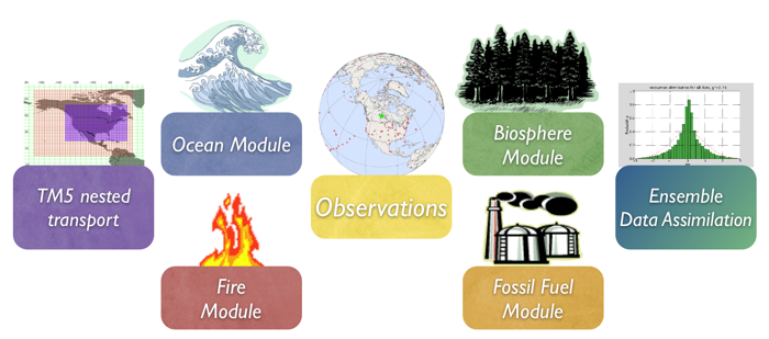
To learn more about a CarbonTracker component, click on one of the above images.
Or download the full PDF version for convenience.
|
|
1. Introduction
Data assimilation is the name of a process by which observations of the 'state' of a system help to constrain the behavior of the system in time. An example of one of the earliest applications of data assimilation is the system in which the trajectory of a flying rocket is constantly (and rapidly) adjusted based on information of its current position to guide it to its exact final destination. Another example of data assimilation is a weather model that gets updated every few hours with measurements of temperature and other variables, to improve the accuracy of its forecast for the next day, and the next, and the next. Data assimilation is usually a cyclical process, as estimates get refined over time as more observations about the "truth" become available. Mathematically, data assimilation can be done with any number of techniques. For large systems, so-called variational and ensemble techniques have gained most popularity. Because of the size and complexity of the systems studied in most fields, data assimilation projects inevitably include supercomputers that model the known physics of a system. Success in guiding these models in time often depends strongly on the number of observations available to inform on the true system state.
In CarbonTracker, the model that describes the system contains relatively simple descriptions of biospheric and oceanic CO2 exchange, as well as fossil fuel and fire emissions. In time, we alter the behavior of this model by adjusting a small set of parameters as described in the next section.
2. Detailed Description
The four surface flux modules drive instantaneous CO2 fluxes in CarbonTracker according to:
F(x, y, t) = λ • Fbio(x, y, t) + λ • Foce(x, y, t) + Fff(x, y, t) + Ffire(x, y, t)
Where λ represents a set of linear scaling factors applied to the fluxes, to be estimated in the assimilation. These scaling factors are the final product of our assimilation and together with the modules determine the fluxes we present in CarbonTracker. Note that no scaling factors are applied to the fossil fuel and fire modules.
2.1 Land-surface classification
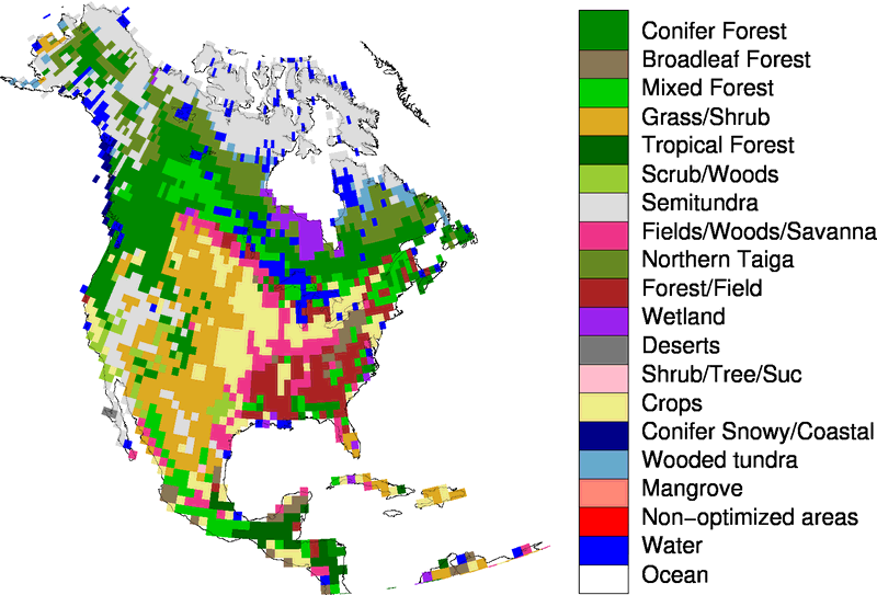
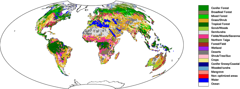
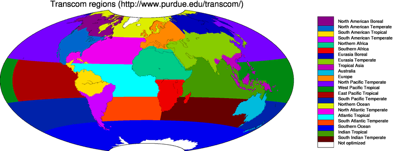
The scaling factors λ are estimated for each week and assumed constant over this period. Each scaling factor is associated with a particular region of the global domain, and currently the geographical distribution of the regions is fixed. The choice of regions is a strong a-priori constraint on the resulting fluxes and should be approached with care to avoid so-called "aggregation errors" [Kaminsky, 1999]. We chose an approach in which the ocean is divided up into 30 large basins encompassing large-scale ocean circulation features, as in the TransCom inversion study (e.g. Gurney et al., [2002]). The terrestrial biosphere is divided up according to ecosystem type as well as geographical location. Thereto, each of the 11 TransCom land regions contains a maximum of 19 ecosystem types summarized in the table below. The figure shows ecoregions for North America (click here for global land ecoregions). Note that there is currently no requirement for ecoregions to be contiguous, and a single scaling factor can be applied to the same vegetation type on both sides of a continent. Further details on ecoregions can be found here.
Theoretically, this approach leads to a total number of 11*19+30=239 optimizable scaling factors λ each week, but the actual number is 156 since not every ecosystem type is represented in each TransCom region, and because we decided not to optimize parameters for ice-covered regions, inland water bodies, and desert. The total flux coming out of these last regions is negligibly small. It is important to note that even though only one parameter is available to scale, for instance, the flux from coniferous forests in Boreal North America, each 1° x 1° grid box predominantly covered by coniferous forests will have a different flux F(x,y,t) depending on local temperature, radiation, and CASA modeled monthly mean flux.
Ecosystem types considered on 1° x 1° for the terrestrial flux inversions is based on Olson, [1992]. Note that we have adjusted the original 29 categories into only 19 regions. This was done mainly to fill the unused categories 16,17, and 18, and to group the similar (from our perspective) categories 23-26+29. The table below shows each vegetation category considered. Percentages indicate the area associated with each category for North America rounded to one decimal.
Ecosystem Types
| category | Olson V 1.3a | Percentage area
|
|---|
| 1 | Conifer Forest | 19.0%
| | 2 | Broadleaf Forest | 1.3%
| | 3 | Mixed Forest | 7.5%
| | 4 | Grass/Shrub | 12.6%
| | 5 | Tropical Forest | 0.3%
| | 6 | Scrub/Woods | 2.1%
| | 7 | Semitundra | 19.4%
| | 8 | Fields/Woods/Savanna | 4.9%
| | 9 | Northern Taiga | 8.1%
| | 10 | Forest/Field | 6.3%
| | 11 | Wetland | 1.7%
| | 12 | Deserts | 0.1%
| | 13 | Shrub/Tree/Suc | 0.1%
| | 14 | Crops | 9.7%
| | 15 | Conifer Snowy/Coastal | 0.4%
| | 16 | Wooded tundra | 1.7%
| | 17 | Mangrove | 0.0%
| | 18 | Non-optimized areas (ice, polar desert, inland seas) | 0.0%
| | 19 | Water | 4.9%
|
Each 1° x 1° pixel of our domain was assigned one of the categories above bases on the Olson category that was most prevalent in the 0.5° x 0.5° underlying area.
2.2 Ensemble Size and Localization
The ensemble system used to solve for the scalar multiplication factors is similar to that in Peters et al. [2005] and based on the square root ensemble Kalman filter of Whitaker and Hamill, [2002]. We have restricted the length of the smoother window to only five weeks as we found the derived flux patterns within North America to be robustly resolved well within that time. We caution the CarbonTracker users that although the North American flux results were found to be robust after five weeks, regions of the world with less dense observational coverage (the tropics, Southern Hemisphere, and parts of Asia) are likely to be poorly observable even after more than a month of transport and therefore less robustly resolved. Although longer assimilation windows, or long prior covariance length-scales, could potentially help to constrain larger scale emission totals from such areas, we focus our analysis here on a region more directly constrained by real atmospheric observations.
Ensemble statistics are created from 150 ensemble members, each with its own background CO2 concentration field to represent the time history (and thus covariances) of the filter. To dampen spurious noise due to the approximation of the covariance matrix, we apply localization [Houtekamer and Mitchell, 1998] for non-MBL sites only. This ensures that tall-tower observations within North America do not inform on for instance tropical African fluxes, unless a very robust signal is found. In contrast, MBL sites with a known large footprint and strong capacity to see integrated flux signals are not localized. Localization is based on the linear correlation coefficient between the 150 parameter deviations and 150 observation deviations for each parameter, with a cut-off at a 95% significance in a student's T-test with a two-tailed probability distribution.
2.3 Dynamical Model
In CarbonTracker, the dynamical model is applied to the mean parameter values λ as:
λ tb = (λ t-2a + λ t-1 a + λ p ) ⁄ 3.0
Where "a" refers to analyzed quantities from previous steps, "b" refers to the background values for the new step, and "p" refers to real a-priori determined values that are fixed in time and chosen as part of the inversion set-up. Physically, this model describes that parameter values λ for a new time step are chosen as a combination between optimized values from the two previous time steps, and a fixed prior value. This operation is similar to the simple persistence forecast used in Peters et al. [2005], but represents a smoothing over three time steps thus dampening variations in the forecast of λ b in time. The inclusion of the prior term λ p acts as a regularization [Baker et al., 2006] and ensures that the parameters in our system will eventually revert back to predetermined prior values when there is no information coming from the observations. Note that our dynamical model equation does not include an error term on the dynamical model, for the simple reason that we don't know the error of this model. This is reflected in the treatment of covariance, which is always set to a prior covariance structure and not forecast with our dynamical model.
2.4 Covariance Structure
Prior values for λ p are all 1.0 to yield fluxes that are unchanged from their values predicted in our modules. The prior covariance structure Pp describes the magnitude of the uncertainty on each parameter, plus their correlation in space. The latter is applied such that the same ecosystem types in different TransCom regions decrease exponentially with distance (L=2000km), and thus assumes a coupling between the behavior of the same ecosystems in close proximity to one another (such as coniferous forests in Boreal and Temperate North America). Furthermore, all ecosystems within tropical TransCom regions are coupled decreasing exponentially with distance since we do not believe the current observing network can constrain tropical fluxes on sub-continental scales, and want to prevent large dipoles to occur in the tropics.
In our standard assimilation, the chosen standard deviation is 80% on land parameters, and 40% on ocean parameters. This reflects more prior confidence in the ocean fluxes than in terrestrial fluxes, as is assumed often in inversion studies and partly reflects the lower variability and larger homogeneity of the ocean fluxes. All parameters have the same variance within the land or ocean domain. Because the parameters multiply the net-flux though, ecosystems with larger weekly mean net fluxes have a larger variance in absolute flux magnitude.
3. Further Reading
|
|
