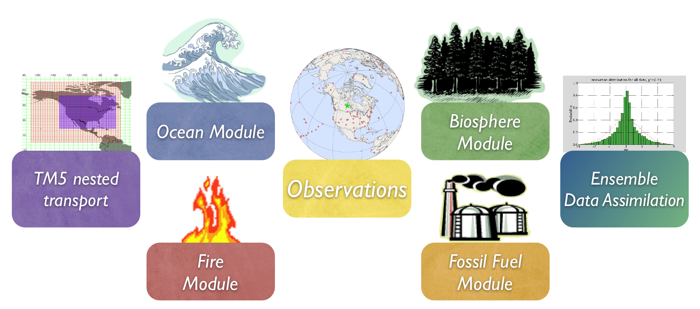
The biosphere model currently used in CarbonTracker is the Carnegie-Ames Stanford Approach (CASA) biogeochemical model. This model calculates global carbon fluxes using input from weather models to drive biophysical processes, as well as satellite observed Normalized Difference Vegetation Index (NDVI) to track plant phenology. The version of CASA model output used so far was driven by year specific weather and satellite observations, and including the effects of fires on photosynthesis and respiration (see van der Werf et al., [2006] and Giglio et al., [2006]). This simulation gives 1x1 degree global fluxes on a monthly time resolution.
Net Ecosystem Exchange (NEE) is re-created from the monthly mean CASA Net Primary Production (NPP) and ecosystem respiration (RE). Higher frequency variations (diurnal, synoptic) are added to Gross Primary Production (GPP=2*NPP) and RE(=NEE-GPP) fluxes every 3 hours using a simple temperature Q10 relationship assuming a global Q10 value of 1.5 for respiration, and a linear scaling of photosynthesis with solar radiation. The procedure is very similar, but NOT identical to the procedure in Olsen and Randerson [2004] and based on ECMWF analyzed meteorology. Note that the introduction of 3-hourly variability conserves the monthly mean NEE from the CASA model. Instantaneous NEE for each 3-hour interval is thus created as:
NEE(t) = GPP(I, t) + RE(T, t)
GPP(t) = I(t) * (∑(GPP) / ∑(I))
RE(t) = Q10(t) * (∑(RE) / ∑(Q10))
Q10(t) = 1.5((T2m-T0) / 10.0)
where T=2 meter temperature, I=incoming solar radiation, t=time, and summations are done over one month in time, per gridbox. The instantaneous fluxes yielded realistic diurnal cycles when used in the TransCom Continuous experiment.
The current CarbonTracker release was based on the CASA runs for the GFED2 project to estimate fire emissions. We found a significantly better match to observations when using this output compared to the fluxes from a neutral biosphere simulation. Due to the inclusion of fires, inter-annual variability in weather
and NDVI, the fluxes for North America start with a small net flux even when no assimilation is done. This flux ranges from 0.05 PgC/yr of release, to 0.15 PgC/yr of uptake.
3. Further Reading