CarbonTracker 2011

CarbonTracker 2011 is the sixth release of the NOAA CO2 measurement and modeling system. CarbonTracker is designed to keep track of sources (emissions to the atmosphere) and sinks (removal from the atmosphere) of carbon dioxide around the world, using atmospheric CO2 observations from a host of collaborators. The current release of CarbonTracker, CT2011, provides global estimates of these surface fluxes of CO2 from January 2000 through December 2010.

Notice: methodological changes   CarbonTracker 2011 is a unique release due to the use of multiple models to provide flux prior guesses. Details are below.

Estimates of CO2 sources and sinks over North America
From 2001 through 2010, ecosystems in North America have been a net sink of 0.7 ± 1.3 PgC yr-1 (1 Petagram Carbon equals 1015 gC, or 1 billion metric ton C, or 3.67 billion metric ton CO2). This natural sink offsets about one-third of the emissions of about 1.9 PgC yr-1 from the burning of fossil fuels in the U.S.A., Canada and Mexico combined (Figure 1).

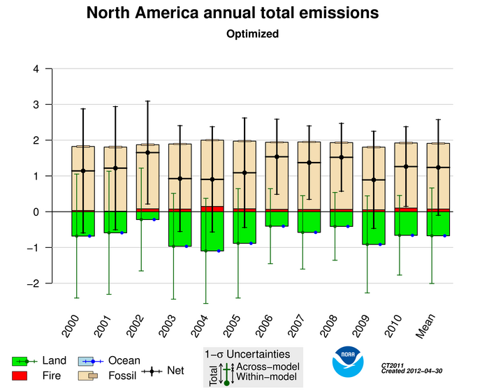
Figure 1. Annual total emissions from North America. The bars in this figure represent CO2 emissions for each year in PgC yr-1 from the U.S.A., Canada, and Mexico combined. See map on this page. CarbonTracker models four types of surface-to-amosphere exchange of CO2, each of which is shown in a different color: fossil fuel emissions (tan), terrestrial biosphere flux excluding fires (green), direct emissions from fires (red), and air-sea gas exchange (blue). Negative emissions indicate that the flux removes CO2 from the atmosphere. The net surface exchange, computed as the sum of these four components, is shown as a thick black line.

The year with the smallest annual uptake by terrestrial ecosystems in North America was 2002, when there was widespread drought in the U.S. west. During this year, land ecosystems accounted for a sink of only 0.2 PgC yr-1. This reduced land sink is largely responsible for 2002 being the year in the CarbonTracker record with the largest input of CO2 to the atmosphere from North America, when net emissions reached 1.7 ± 0.6 PgC yr-1.

In contrast, our observing system did not detect an effect from the 2007 drought in the U.S. Southeast. This is likely due to lack of coverage of the area (Figure 3) in our current observing network. New observations in CT2011 compared to CT2009, however, do lead to interesting differences in this region for 2008. For CT2011 in 2008, the U.S. Southeast represents a distinct source of carbon dioxide to the atmosphere, whereas CT2009 fluxes for this same place and time are equivocal.

In CT2011, we find that 2003, 2004, and 2009 were the years with the largest North American land sink, with ecosystems taking up about 0.9 - 1.1 PgC yr-1—a land sink that is about 36% bigger than the average. Fossil fuel emissions from North America were also slightly reduced in 2009 compared to earlier years as a result of the economic downturn. As a result, ecosystems removed about half of fossil fuel emissions over North America in 2009, and this was the year with the lowest net input of CO2 to the atmosphere from North America. This 2009 net annual emission was 0.9 ± 1.4 PgC yr-1, about 25% smaller than the average of 1.2 ± 1.1 PgC yr-1. This is the first year since the beginning of the CarbonTracker record in 2000 for which the net flux from North America has fallen below 1 PgC yr-1.

Spatial distribution of surface fluxes
CarbonTracker flux estimates include sub-continental patterns of sources and sinks coupled to the distribution of dominant ecosystem types across the continent (Figure 2). We have greater confidence in countrywide totals than in estimates of regional sources and sinks, but we expect that such finer-scale estimates will become more robust with future expansion of the CO2 observing nework. Our results indicate that the sinks are mainly located in the agricultural regions of the Midwest (36%), deciduous forests along the East Coast (33%), and boreal coniferous forests (17%).

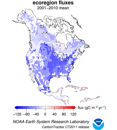Figure 2. Mean ecosystem fluxes. The pattern of net ecosystem exchange (NEE) of CO2 of the land biosphere averaged over 2001-2009, as estimated by CarbonTracker. This NEE represents land-to-atmosphere carbon exchange from photosynthesis and respiration in terrestrial ecosystems, and a contribution from fires. It does not include fossil fuel emissions. Negative fluxes (blue colors) represent CO2 uptake by the land biosphere, whereas positive fluxes (red colors) indicate regions in which the land biosphere is a net source of CO2 to the atmosphere. Units are gC m-2 yr-1.

Since CarbonTracker simulates CO2 throughout the entire atmospheric column, the model atmosphere can be sampled exactly like satellite retrievals of CO2. Such estimates are generally more sensitive to the CO2 mole fraction in some parts of the atmosphere than in others, and by using a vertical profile of this sensitivity, a direct analog of the satellite estimate can be constructed.

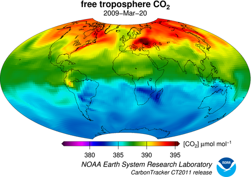
Figure 4. Carbon dioxide weather Shown is the daily average of the pressure-weighted mean mole fraction of carbon dioxide in the free troposphere as modeled by CarbonTracker for March 20, 2009. Units are micromoles of CO2 per mole of dry air (μmol mol-1), and the values are given by the color scale depicted under the graphic. The "free troposphere" in this case is levels 6 through 10 of the TM5 model. This corresponds to about 1.2km above the ground to about 5.5km above ground, or in pressure terms, about 850 hPa to about 500 hPa. Gradients in CO2 concentration in this layer are due to exchange between the atmosphere and the earth surface, including fossil fuel emissions, air-sea exchange, and the photosynthesis, respiration, and wildfire emissions of the terrestrial biosphere. These gradients are subsequently transported by weather systems, even as they are gradually erased by atmospheric mixing.

Furthermore, the estimates do not take into account several additional factors noted below. The calculation is set up for sources and sinks to slowly revert, in the absence of observational data, to first guesses of net ecosystem exchange, which are close to zero on an annual basis. This set-up may result in a bias. Also due to the sparseness of measurements, we have had to assume coherence of ecosystem processes over large distances, giving existing observations perhaps an undue amount of weight. The process model for terrestrial photosynthesis and respiration was very basic, and will likely be greatly improved in future releases of CarbonTracker. Easily the largest single annual mean source of CO2 is emissions from fossil fuel burning, which are currently not estimated by CarbonTracker. We use estimates from emissions inventories (economic accounting) and subtract the CO2 mole fraction signatures of those fluxes from observations. As a result, the biosphere and ocean fluxes estimated by CarbonTracker inherit error from the assumed fossil fuel emissions. While these emissions inventories may have a small relative error on global scales (perhaps 5 or 10%), any such bias translates into a larger relative error in the annual mean ecosystem sources and sinks, since those fluxes have smaller magnitudes. We expect to add a process model of fossil fuel combustion in future releases of CarbonTracker. Finally, additional measurement sites are expected to lead to the greatest improvements, especially to more robust and specific source/sink results at smaller spatial scales.

Consistency of modeled and observed atmospheric CO2 growth rates
Global atmospheric CO2 growth rates inferred directly from observed carbon dioxide at marine surface sites are consistent with those modeled by CarbonTracker, both in their average values and in their year-to-year variations (Figure 5). These global growth rates continue to hover at around 4 PgC yr-1, or around 1.9 ppm yr-1 (Figure 5). The 2009 growth rate modeled by CarbonTracker was below average at 3.4 ± 3.1 PgC yr-1. This was not due to a significant decrease in fossil fuel emissions, as can be seen from estimates of global fluxes used in CarbonTracker. Instead, the most notable difference for the 2009 atmospheric growth rate appears to be reduced biomass burning fluxes from the tropics and southern hemisphere, which at 1.4 PgC yr-1 are about 0.5 PgC yr-1 below their 2001-2009 mean of 1.9 PgC yr-1.

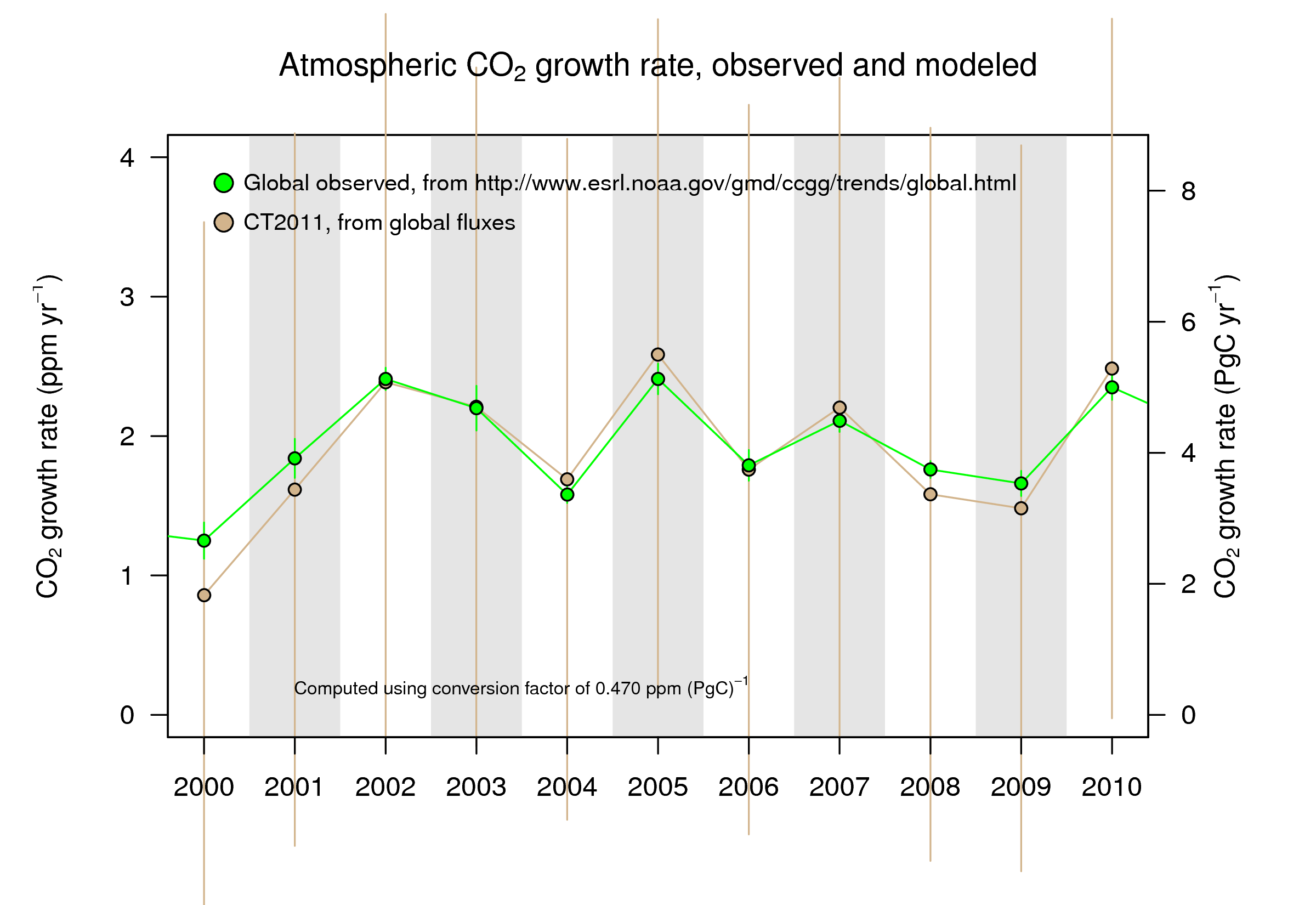
Figure 5. Atmospheric CO2 growth rates. Observed atmospheric CO2 growth rates (source: NOAA ESRL page on global trends in CO2) are plotted against the atmospheric CO2 growth rate inferred from CT2011 global fluxes. Note that error bars on the observed growth rates are relatively small and may not be visible on this plot.

CarbonTracker is a NOAA contribution to the North American Carbon Program