Curve Fitting Methods Applied to Time Series in NOAA GML
The pattern of CO2 measurements (and other gases as well) at locations around the globe show basically a combination of three signals; a long-term trend, a non-sinusoidal yearly cycle, and short term variations that can last from several hours to several weeks, which are due to local and regional influences. Since the objective in many studies of CO2 is to determine the 'background' distribution in the atmosphere without influence by local sources and sinks, a method of filtering or smoothing the data is desired in order to investigate the signals occuring in the record on different time scales.
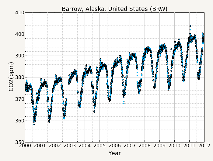
For example, figure 1 shows the CO2 measurement record of daily averages from Barrow, Alaska for the years 2000-2011. The curve fitting used will consist of a function fit to the data, and digital filtering of the residuals from the fit.
A C language program and a Python class for computing the curves described on this page is available at https://gml.noaa.gov/aftp/user/thoning/ccgcrv/
1. Function Fit to the Data
The first step is to fit a function which approximates the annual oscillation and the long term growth in the data. The long term growth is represented by a polynomial function and the annual oscillation is represented by harmonics of a yearly cycle. This function can be fit to the data using methods of general linear least squares regression (that is, linear in its parameters) and can be solved by a variety of routines. The routine used in the program is scipy.optimize.leastsq for python and LFIT (Press et al., 1988) for the C version. This routine also returns the covariances of the parameters so that an estimate of the uncertainty of the fit can be made.

Equation 1: Function fit to the data.
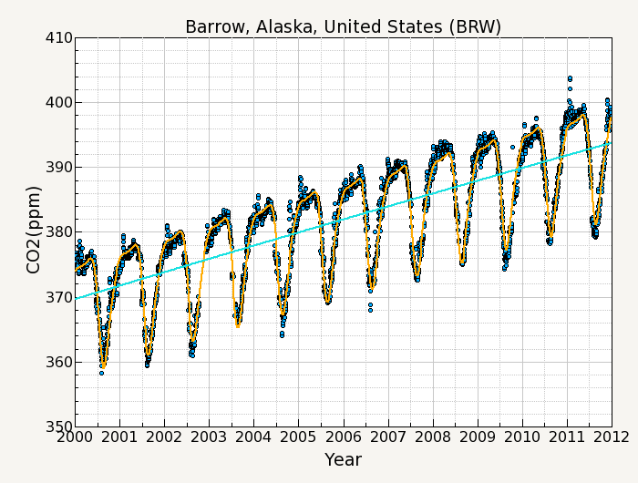
where k is the number of polynomial terms, and nh is the number of harmonics in the function. Typical values used are k=3 polynomial terms (a quadratic) and nh=4 yearly harmonics. Figure 2 shows the function fit to the Barrow data.
2. Filtering of residuals
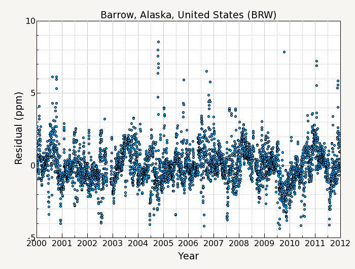
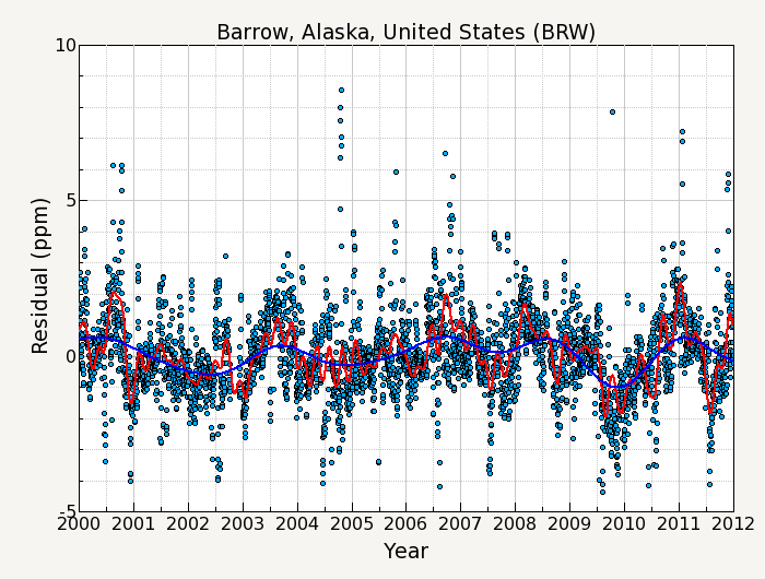
The next step is to calculate and filter the residuals of the original data about the function. These residuals are filtered in order to define interannual and short term variations that are not determined by the function. Figure 3 shows a plot of the residuals from the function fit.
The filtering method is a slight modification of the filter explained by Thoning et al (1989). The method used is to transform the data into the frequency domain using a Fast Fourier Transform (FFT), apply a low pass filter function to the frequency data, then transform the filtered data to the real domain using an inverse FFT.
The major requirement for the FFT algorithm that is used ( scipy.fftpack.rfft or REALFT, Press et al., 1988) requires that the data be equally spaced without gaps. Since the data never satisfies these requirements completely, some form of interpolation is needed. The method used is simple linear interpolation between points. The interval between interpolated data points is specified by the user, and is called the "sampling interval".
Another requirement of the FFT is that the number of points be equal to integral power of 2. This is achived by "zero padding" the data equally at both ends of the record until the correct number of points are obtained. Tests with other fft routines, (fftw, Gnu Scientific Library) which don't require 2p number of points, give identical results to the REALFT routine.
Because this zero padding can affect the ends of the filter, the residuals are corrected so that the ends of the record are approximately zero. This is done by taking approximately ½ year of data at each end of the record (actually the long term cutoff value/4), performing a linear regression on this data, and correcting the residuals by the slope of this line. The data is then transformed to the frequency domain using the FFT algorithm.
The transformed data is multiplied by a low pass filter function (equation 2) where the cutoff frequency fc is chosen so that h(f) = 0.5 at f=fc. The value of fc is the only variable involved for determining the "stiffness" or frequency response of the filter. The residuals are filtered twice, once with a short term cutoff value for smoothing the data, and once with a long term value to remove any remaining seasonal oscillation and to track interannual variations in the data not seen by the polynomial part of equation 1.

Equation 2: Low Pass Filter Function.
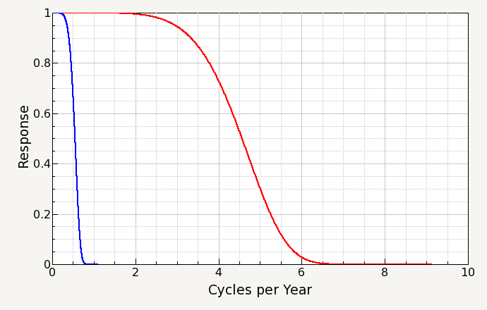
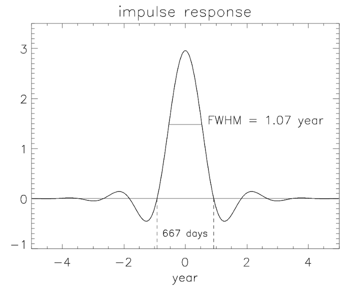
The value for fc is specified in 'number of days'. Figure 4 shows the response function with cutoff values of 80 days for the short term filter and 667 days for the long term filter.
The filtered data is then transformed back to the time domain with an inverse FFT. The correction due to the linear regression to the ends of the data is added back in to get the final filter results. Figure 5 shows the results of applying the filter to the residual data.
3. Statistical Uncertainty of the Function
The variance of the function fit is given by

Equation 3: Error estimate of the Function fit.
 is the partial derivative of the function with
respect to paramter j, and
  is the reduced chi squared value. For the partial
derivatives, we calculate it using a mean value of x.
4. Statistical Uncertainty of the Filter
Filtering with this method in the frequency domain is equivalent to convolution filtering in the time domain [Koopmans, 1974, pp. 180-182]. That is, filtering in the frequency domain can be visualized as a weighted moving average process in the time domain. The weights of this moving average can be determined by the values of the impulse response function (IRF) of the filter transfer function. The IRF is the inverse transform of the filter transfer function and is a measure of how the filter responds to a delta function impulse in the time domain. Figure 6 shows the IRF of the exponential filter for the cutoff point at 667 days. The full width at half maximum (FWHM) for the 667 day cutoff is 1.07 years, The FWHM of the response function for the 80 day cutoff is 47 days.
We can use this formulation of the filter in the time domain to facilitate estimation of the statistical uncertainty associated with the filtered time series. The variance of the result of the filter is calculated using equation 3.

Equation 4: Error estimate of the Low Pass Filter Function.
where ci are the filter weights, and r(k-j) are the lags in a first-order auto regressive process r(k) = r(1)k ,k =1,2,... The terms in equation 4 are then the variance of the residuals about the filter, the sum of the squares of the filter weights, and the covariance between data points, which takes into account serial correlation in the data.
5. Determination of component signals
At this point, all curve fitting has been completed. It is now just a matter of combining the appropriate parts of the function and the filter to derive the signal component of interest. The components of most interest and how they are defined are:
- Smoothed data - Curve with only the shortest term variations removed. This is the function fit plus the filtered residuals using the short term cutoff value.
- Trend - Upward growth in the data with the seasonal cycle removed. This is the polynomial part of the function fit plus the filtered residuals using the long term cutoff value.
- Detrended seasonal cycle - Annual oscillation with trend removed. This is the annual harmonic part of the function fit plus the filtered residuals using the short term cutoff value.
- Seasonal amplitude - Magnitude of the peak to trough of the detrended seasonal cycle.
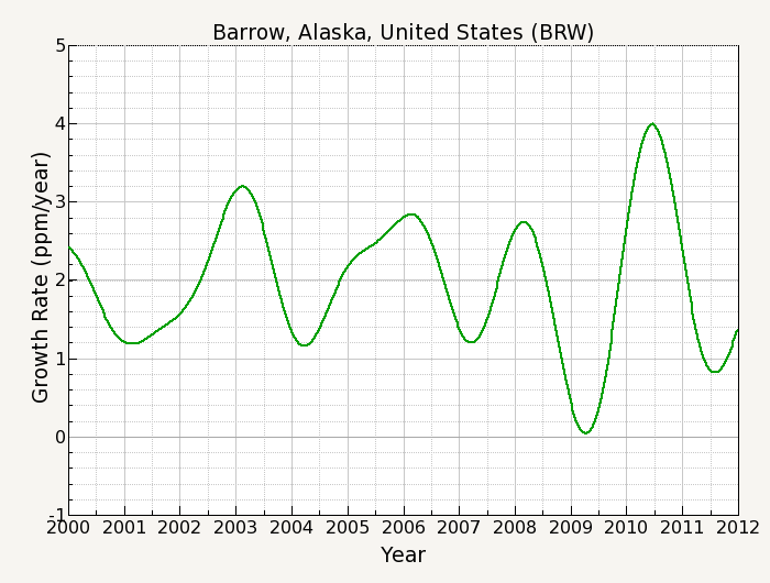
- Growth rate - Rate of increase (first derivative) of the trend.
Smoothed Data
Each of the components can be determined from the results of the function fit and the filtering of the residuals. The smoothed curve is obtained by combining the results of the function and the results of the filter using the short term cutoff value. The variance of a point on this curve is given by combining the variances of the function and the filter

Equation 5: Error estimate of the smoothed data.
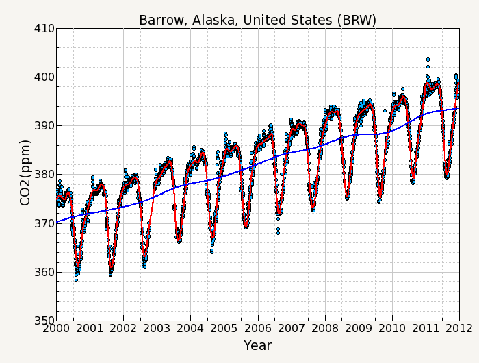
The smoothed data is shown as the red line in figure 7.
Trend Data
The trend curve is obtained by combining only the polynomial part of the function with the results of the filter using the long term cutoff value. The variance of the trend is obtained by combining the variance of the function with the variance of the filter using the long term cutoff value:

Equation 6: Error estimate of the trend data.
To be conservative, this program assumes that 
The trend data is shown as the blue line in figure 7.
Detrended Seasonal Cycle
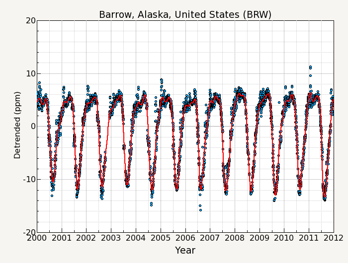
The detrended seasonal cycle is obtained by subtracting the trend curve from the smooth curve. The variance of this curve is obtained by combining the appropriate variances

Equation 7: Error estimate of the detrended annual cycle.
The seasonal amplitude for each year is determined by finding the maximum value of the detrended cycle minus the minimum value of the detrended cycle. The variance of the amplitude is then

Equation 8: Error estimate of the seasonal amplitude.
Growth Rate
The growth rate is determined by taking the derivative of the trend curve. Because the trend is made up of discrete points rather than in a functional form, a numerical method for calculating the derivative is needed. In practice, an interpolating cubic spline curve is computed which passes through each trend point, with the derivative of the spline at each trend point also computed. The derivative is approximately equivalent to taking the difference of two points one year apart and plotting this difference midway between the two points. Thus the variance of the growth rate is given by

Equation 9: Error estimate of the growth rate.
6. Conclusion
There are a few things to be aware of when using this curve fitting method. For less than 3 years of data it is best to use a linear term for the polynomial part of the function (k=2). This will keep the polynomial part of the function from being unduly influenced by the seasonal cycle in the data. Because the function fit is a least-squares fit, it is sensitive to outliers. There can also be problems handling large gaps in the data for the filter step. If the data points before and/or after the gap are 'outliers', the interpolation over the gap may not accurately represent what the true data might have been.
The FFT filter can produce end effects if the residuals from the function depart significantly from 0 at the ends of the record. This is the reason why the residuals are corrected by a linear fit to the ends of the data before the FFT is performed. This especially affects the growth rate at the ends of the record. To get an idea of the uncertainty in the growth rate, try different values for the number of polynomial terms and observe the differences.
The advantages of this method are that the harmonic coefficients are valuable as a definition of the annual cycle and can be compared to harmonics generated by carbon cycle models. The harmonic function is good for handling relatively large gaps in the data (but the filter step may have problems as mentioned in the paragraph above). The curve also captures the point of deepest drawdown in the summer of the northern hemisphere sites without introducing spurious variability in other parts of the record. The combination of harmonics and filtered residuals allows the curve to follow changes in the shape of the seasonal cycle and interannual variations in the long term trend. This method works equally well with either high frequency in-situ data or relatively low frequency flask sampling data. Only correct values for the sampling interval and the filter cutoff are required for either data set.
References
- Thoning, K.W., P.P. Tans, and W.D. Komhyr, 1989, Atmospheric carbon dioxide at Mauna Loa Observatory, 2. Analysis of the NOAA/GMCC data, 1974 1985., J. Geophys. Res. ,94, 8549 8565.
- Press, WH; Teukolsky, SA; Vetterling, WT; Flannery, BP 1988, Numerical Recipes in C: The Art of Scientific Computing (1st ed.), New York: Cambridge University Press
- Koopmans, L.H. 1974, The Spectral Analysis of Time Series, Academic, San Diego, Calif.
