How we measure background CO₂ levels on Mauna Loa.

Pieter Tans and Kirk Thoning, NOAA Earth System Research Laboratory,
Boulder, Colorado
September, 2008. Updated December, 2016; March 2018

Summary

We have confidence that the CO₂ measurements made at the Mauna Loa Observatory reflect truth about our global atmosphere. The main reasons for that confidence are:

1. The Observatory near the summit of Mauna Loa, at an altitude of 3400 m, is well situated to measure air masses that are representative of very large areas.
2. All of the measurements are rigorously and very frequently calibrated.
3. Ongoing comparisons of independent measurements at the same site allow an estimate of the accuracy, which is generally better than 0.2 ppm.

Infrared absorption.

How does the CO₂ analyzer work?

Air is slowly pumped through a small cylindrical cell with flat windows on both ends. Infrared light is transmitted through one window, through the cell, through the second window, and is measured by a detector that is sensitive to infrared radiation. In the atmosphere carbon dioxide absorbs infrared radiation, contributing to warming of the earth surface. Also in the cell CO₂ absorbs infrared light. More CO₂ in the cell causes more absorption, leaving less light to hit the detector. We turn the detector signal, which is registered in volts, into a measure of the amount of CO₂ in the cell through extensive and automated (always ongoing) calibration procedures.

Mole fraction in dry air

What do we need to measure?

Most people assume that we measure the concentration of CO₂ in air, and in communicating with the general public we frequently use that word because it is familiar. The quantity we actually determine is accurately described by the chemical term “mole fraction”, defined as the number of carbon dioxide molecules in a given number of molecules of air, after removal of water vapor. For example, 372 parts per million of CO₂ (abbreviated as ppm) means that in every million molecules of (dry) air there are on average 372 CO₂ molecules. The table below gives an example for 372 ppm CO₂ in dry air (this is roughly the average amount of CO₂ in the atmosphere in the beginning of the year 2002). All species have been expressed as ppm, turning 78.09% nitrogen into 780,900 ppm. The rightmost column shows the composition of the same air after 3% water vapor has been added:

	dry air	3% wet air
Nitrogen	780,900	757,473 ppm
Oxygen	209,400	203,118
Water vapor	0	30,000
Argon	9,300	9,021
Carbon Dioxide	372	360.8
Neon	18	17.5
Helium	5	4.9
Methane	2	2
Krypton	1	1
trace species (each less than 1)	1	1
Total	1,000,000	1,000,000 ppm

Why do we express the abundance of CO₂ as a mole fraction in dry air?

The concentration of a gas is defined formally as the number of molecules per cubic meter. The goal of our measurements is to quantify how much CO₂ has been added to, or removed from, the atmosphere. The concentration does not give us that information because it primarily depends on the pressure and temperature, and secondarily on how much the relative abundance of each gas has been diluted by water vapor, which is extremely variable. Only the dry mole fraction reflects the addition and removal of a gas species because its mole fraction in dry air does not change when the air expands upon heating or upon ascending to higher altitude where the pressure is lower. Nor does it change when water evaporates, or condenses into droplets. Why is this so important? Here is an example: The amount of CO₂ is higher in the Northern than in the Southern Hemisphere as a result of the combustion of coal, oil, and natural gas. The measurement of this difference gives us crucial quantitative information about the emissions and removals of CO₂. The concentration change produced by the addition of water vapor can be greater than the CO₂ difference between the two hemispheres. In contrast, the difference in dry mole fraction does reflect the differences in emissions and removals between the hemispheres.

One often encounters in the literature the term “mixing ratio”. This is ambiguous. Does it apply to mass or to the numbers of molecules? In an attempt to clear that up one also often finds “mixing ratio by volume”, abbreviated as “ppmv” for CO₂. However, that can still be ambiguous. Does it mean partial molar volume of CO₂ relative to molar volume of whole air? That would only be correct if all the constituent gases of air behaved as ideal gases, which we know is not true. Furthermore, the calibration standards used for greenhouse gases in air are made as, and expressed as, mole fractions in (dry) air. All national metrology institutes, with NOAA/ESRL representing the WMO Global Atmosphere Watch community (see gml.noaa.gov/ccl/ ), participate in comparisons of reference gas standards that are called “Key Comparisons of Amount of Substance Ratios”. The unit of “amount of substance” is the mole.

Data Availability

The CO₂ data that is described on this page is available at the GML Data Finder, where data options have been filtered to show CO₂ data from all of the GML Observatories (In addition to Mauna Loa, Barrow Alaska, American Samoa and South Pole are included). Data is available as hourly, daily and monthly averages.

Calibration of the instrument.

The most important aspect of the measurements is the ongoing calibrations. Air flows continually through the instrument, after having first been dried in a cold trap where the water vapor freezes out as ice on the walls. Unfortunately, the absorption that we measure in the cell does not depend on the CO₂ mole fraction, but on the total amount of CO₂ in the cell. Therefore, we either have to extremely accurately control the temperature and pressure in the cell, as well as the flow rate, or we can control them less accurately while using frequent calibrations of the instrument with reference gas mixtures of CO₂-in-dry-air spanning the expected range of the measurements. The reference gas mixtures are stored in high pressure aluminum cylinders. At Mauna Loa the calibration is done every hour by interrupting the flow of outside air through the cell, and replacing it with flows of three reference gas mixtures in succession, 5 minutes each. An example is shown in Figure 1. Each hour is divided up as follows:

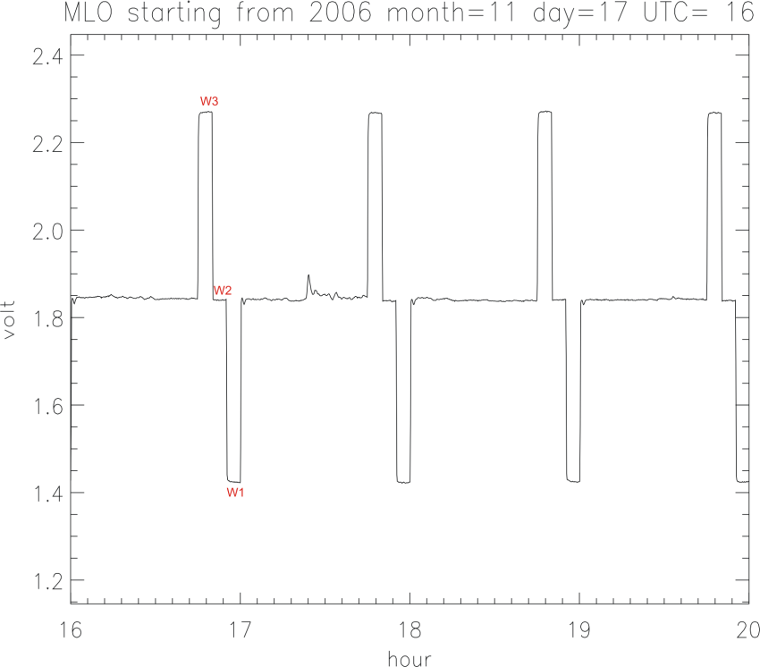
• minute 0 through 24: air intake line 1 (last 20 minutes is used)
• minute 25-44: air intake line 2 (20 minutes used)
• minute 45-49: high reference gas, which we call W3 (last 2 minutes is used)
• minute 50-54: middle reference gas (W2) (last 2 minutes is used)
• minute 55-59: low reference gas (W1) (last 2 minutes is used)

We know the mole fractions of CO₂ in the reference gases very accurately. In this case they were 370.50 ppm (W1), 379.93 (W2), and 389.72 (W3). For each of these three we register a voltage, which establishes a relationship between voltage and CO₂ mole fraction. The relationship is not linear because the sensitivity of the detector decreases at higher CO₂ abundance, although the effect is not strong in the small range measured at Mauna Loa. We fit a quadratic function through the three points to provide a CO₂ mole fraction number for every voltage in the range shown in Figure 1, from ~1.4 to ~2.3 volt. After each gas switch the first few minutes are ignored to eliminate switching transients. For example, the flow rate is 100 cc per minute, and it takes time for the previous air to be fully replaced with new air, and for the walls of the tubes, valves, and cell to equilibrate with the new mole fraction. During minutes 0 through 44 we use two separate air intake lines in succession, both from the top of a 38 m tall tower next to the observatory, to facilitate detection of a potential leak between in the intake lines bewteen the tower and the instrument. The tower was built to eliminate any influence on the measurements of human activities at the observatory.

Target gas.

The calibration strategy outlined above can be applied, with appropriate variations, to any separation/detection method, whether it is infrared absorption, gas chromatography, mass spectrometry, etc. Therefore the choice of measurement method is mostly one of convenience. The measurement results do depend very strongly on the control of the reference gas mixtures. If one of them has the wrong value, all results will be off. We provide for a check on the assigned values of the calibration mixtures by running what we call a “target gas”, treated as having an unknown mole fraction, every 25 hours through the measurement system. In reality the mole fraction of the target gas is very accurately known.

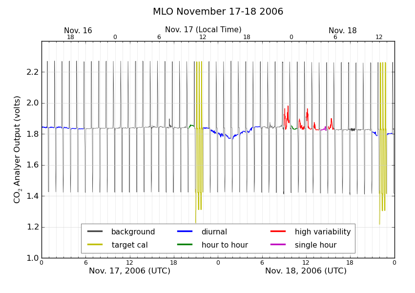
If one of the calibration gases has a wrongly assigned value the measurement of the target gas will produce the wrong result. An example of a daily target measurement is shown in Figure 2 where, during hour 21, the analyzer alternates between the three calibration gases and the target gas. The target gas has low mole fraction in this case, registering at ~1.3 volts. The repeat cycle of every 25 hours causes the target measurement to slowly move through the diurnal cycle because every day it is measured one hour later than on the previous day.

Data selection for background air.

In 1957 Dave Keeling, who was the first to make accurate measurements of CO₂ in the atmosphere, chose the site high up on the slopes of the Mauna Loa volcano because he wanted to measure CO₂ in air masses that would be representative of much of the Northern Hemisphere, and, hopefully, the globe. That goal has not changed. We still want to eliminate the influence of CO₂ absorbed or emitted locally by plants and soils, or emitted locally by human activities. Dave Keeling also introduced the principle of a rigorous calibration strategy that we still employ today.

The observatory is surrounded by many miles of bare lava, without any vegetation or soil. This provides an opportunity to measure “background” air, also called “baseline”” air, which we define as having a CO₂ mole fraction representative of an upwind fetch of hundreds of km. Nearby emission or removal of CO₂ typically produces sharp fluctuations, in space and time, in mole fraction. These fluctuations get smoothed out with time and distance through turbulent mixing and wind shear. A distinguishing characteristic of background air is that CO₂ changes only very gradually because the air has been mixed for days, without any significant additions or removals of CO₂. Another common word for emissions is “sources”, and for removals, “sinks”.

Figure 2 shows an example of the data selection procedures we use to categorize air that has likely been influenced significantly by nearby sources/sinks. The plot is for two days, November 17 and 18, 2006. First the time axis needs to be explained. The bottom axis of Figure 2 reflects that we keep date and time at the Mauna Loa Observatory in Universal Coordinated Time, abbreviated as UTC. UTC is the same across the entire world. It succeeded Greenwich Mean Time in 1961, and is widely used and unambiguous. Local time in Hawaii lags UTC by 10 hours, so that 10 am UTC corresponds to midnight locally. The upper axis has labels indicating the local time in Hawaii.

At Mauna Loa we use the following data selection criteria:

1. The standard deviation of 10-second averages should be less than 0.30 ppm within a given hour. A standard deviation larger than 0.30 ppm is indicated by a “V” flag in the hourly data file, and by the red color in Figure 2.

2. There is often a diurnal wind flow pattern on Mauna Loa driven by warming of the surface during the day and cooling during the night. During the day warm air flows up the slope, typically reaching the observatory at 9 am local time (19 UTC) or later. The upslope air may have CO₂ that has been lowered by plants removing CO₂ through photosynthesis at lower elevations on the island, although the CO₂ decrease arrives later than the change in wind direction, because the observatory is surrounded by miles of bare lava. Upslope winds can persist through ~7 pm local time (5 UTC, next day, or local hour 19 in Figure 2). Hours that are likely affected by local photosynthesis (11am to 7pm local time, 21 to 5 UTC) are indicated by a “U” flag in the hourly data file, and by the blue color in Figure 2.

   At night the flow is often downslope, bringing background air. However, that air is sometimes contaminated by CO₂ emissions from the crater of Mauna Loa. As the air meanders down the slope that situation is characterized by high variability of the CO₂ mole fraction. In Figure 2, downslope winds resumed on November 18 at hour 5 UTC. Hour 9 UTC on the 18^th in Figure 2 is the first of an episode of high variability lasting 7 hours.

3. In keeping with the requirement that CO₂ in background air should be steady, we expect the hourly average from one hour to the next should not differ from the preceding hour by more than a small amount. Data where this hour-to-hour change exceeds 0.25 ppm is indicated by a 'D' flag in the hourly data file, and by the green color in Figure 2. However, if there are 3 consecutive non-flagged hours that either preceed or follow an hour with a 'D' flag, then the 'D' flag is removed. This handles a 'step' change in CO₂ concentration, where the edges of the step agree with surrounding hours, but not with the single adjacent hour.

4. After the application of the 'V', 'U' and 'D' flags, there can be times when a single hour remains unflagged, but is bracketed by flagged data. This makes it unclear if this single hour could be representative of background air or not. We therefore apply a 'S' flag to these single hours. Hour 14 UTC on November 18 in Figure 2 is an example of this. Similarly, a pair of hourly data could be bracketed by flagged data. As a final step, we check if there are any unflagged data within ± 8 hours of an hourly average, ignoring adjacent hours. If not, then that hour is given a 'N' flag.

Hours for which we do not have valid air measurement are flagged with either a '*' or 'I' character in the hourly data file. The hours during which we do a target gas measurement are an example, but there are also other instrumental causes, such as mechanical problems with pumps and valves.

The frequency for each of these flags for a typical year (2014) is shown in Table 1.

Table 1. Number of hours in 2014 for each flag that was applied to the data.

Flag	Number of Hours	Percentage of year*
No flag	3323	37.9%
V	578	6.6%
U	2680	30.6%
D	1063	12.1%
S	232	2.6%
N	34	0.4%
* or I	858	9.8%
*There are 8760 hours in the year.

Hourly means are calculated wherever possible, and how we use that data is indicated by the selection flags. No data are thrown away. The hourly averages are calculated from the 'raw' data, which are the voltages recorded for the air measurements as well as for the reference gas mixtures used for calibration and for the target gas.

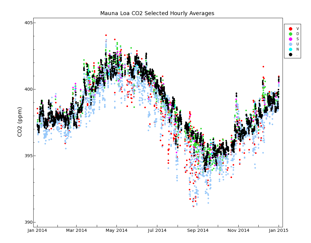
On average over the entire record there are 9.0 retained hours per day with background CO₂ mole fractions. Because of the upslope wind condition flag 'U', there is only a maximum of 15 hours per day of background values possible. Figure 3 show a plot of the CO₂ data for 2014 for each flag type. Even though the data selection method identifies background data properly most of the time, there can still be conditions where the applied selection flag is not approriate. The user of the data should be aware of this and modify the selection as needed.

Auxiliary measured variables

System status variables measured and continuously recorded are: analyzer temperature, cold trap temperature, room temperature, sample flow rate, and both pressure and flow rate through both air intake lines from the tower.

How we calibrate the reference gases.

Since 1995 our laboratory has been the CO₂ Central Calibration Laboratory of the World Meteorological Organization (WMO). Before 1995 that role was filled by the Scripps Institution of Oceanography of the University of California in San Diego. We maintain the WMO Mole Fraction Scale for CO₂-in-air. The WMO Scale is based on 15 so-called Primary Standards that are calibrated in terms of fundamental quantities at intervals of ~1.5 year by manometric measurements. They have CO₂ mole fractions that span the range of ambient air. The primaries are stored in high pressure aluminum cylinders. The Primary Standards themselves are only sparingly used, so that we can build up a calibration history for each of them over several decades.

During a calibration episode, lasting 2-3 months, each Primary is measured three times. Each time a sample of air is taken from the cylinder and its pressure and temperature inside a closed volume are measured very accurately, after temperature and pressure have stabilized in a temperature controlled environment. The volume of approximately 6 liters is accurately known. Once the pressure, temperature, and volume of a gas are known, the amount of gas can be calculated, taking the temperature dependent compressibility of the gases into account. Then the air, with the CO₂ that is to be determined still in it, is slowly and completely flowed at low pressure over a cold trap cooled with liquid nitrogen. The condensate in the cold trap consists of carbon dioxide, nitrous oxide, and residual water vapor. The latter is low, corresponding to 1 ppm or so in the dry high pressure cylinder. After separation of the water vapor component, the carbon dioxide and nitrous oxide are transferred to a small volume, about 10 cc, which has also been very accurately calibrated. After stabilization, the pressure and temperature are once again recorded, and total amount of the two remaining gases calculated. At that point we have determined the combined mole fraction of carbon dioxide and nitrous oxide in the cylinder air. The latter typically comprises less than one thousandth of the total, and we correct for its contribution after measuring nitrous oxide separately on a gas chromatograph.

The accuracy of the WMO Scale has been estimated, based on the accuracy of the temperature, volume and pressure measurement, and the gas handling procedures, at 0.07 ppm. It has been compared several times to calibration scales established independently by other laboratories that were based on weighing a small amount of pure carbon dioxide that was then mixed into a large, also accurately weighed, amount of carbon dioxide-free air. We have also compared to the previous WMO Scale maintained by Scripps. These comparisons are compatible with our internal accuracy estimate.

The manometric calibrations are a very time consuming process, while we need to calibrate thousands of cylinders, many of which are used by other laboratories around the world. We transfer, or propagate, the WMO scale to other high pressure cylinders of CO₂-in-air in a much more efficient way, by comparing them to each other on an infrared gas analyzer system. This is very similar to how we measure outside air by comparing the voltage response of unknown air to the response of air with known mole fractions. The repeatability of these transfer calibrations, done one week or more apart, is typically 0.01-0.02 ppm in the range of ambient air. The sequence is similar to that of target gas calibrations at the field observatories where all cylinders are measured repeatedly, one after the other, with the known gases interspersed between the unknown gases. Because we want to use the Primary Standards sparingly, we transfer the scale twice per year through these comparisons to Secondary Standards, which in turn get used to calibrate all other reference gases. The Secondaries typically last for 3-5 years.

An important aspect of the calibration strategy is that reference gas mixtures are not only calibrated before use, but also after their use when the pressure is low, but not close to zero. Reference gas mixtures are recalled for recalibration when ~20% of the air is still in the cylinder because experience has shown that the CO₂ mole fraction tends to drift more when the pressure becomes low. Because the raw data consists of voltages, it is possible to re-calculate corrected mole fractions for the measured atmospheric air after it has become clear through recalibration that a particular reference gas has drifted. Fortunately this problem greatly diminished when we made the switch from using steel cylinders to aluminum cylinders.

Replication of the field measurements

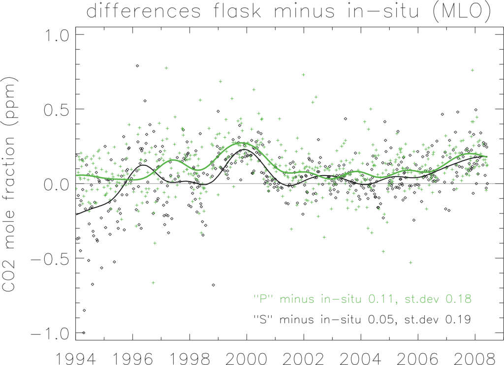
We know from experience that careful calibration is necessary, but not sufficient, for making accurate measurements. There are many potential biases related to gas handling, drying, that are not covered through the calibration. The ultimate test of how accurate these measurements are likely to be is to compare them with other measurements, done independently, with different methods, and/or by different laboratories. At Mauna Loa we have both. In Figure 4 we show a comparison with two sets of grab samples of air in glass flasks, done weekly in pairs. One set, called “S”, are samples taken through the intake line used by the continuous analyzer, and diverted just before entering the analyzer. The second set, called “P”, are completely independent from the continuous analyzer system. They are taken with a battery operated pump, and extendable air intake mast, at a spot on the roof of one of the observatory buildings. The flask samples are sent to our laboratory in Boulder, Colorado, where they are analyzed together with thousands of other air samples from all over the world. There is a fair amount of “scatter” in the comparisons, partly because we are comparing a spot sample, a ~20 s average, to the hourly average of the continuous analyzer when the sample was taken. On average, the “P” flasks differ from the continuous analyzer by 0.11 ppm, and the “S” flasks by 0.05 ppm. Important are systematic biases that persist over a good part of a year and more, portrayed by the solid smooth lines fitted to the respective data sets. One can see that most of the time the biases are less than 0.2 ppm.

We have a similar comparison with the CO₂ measurements performed by the Scripps Institution of Oceanography, the program started by David Keeling. They have always maintained their own manometric calibration scale, they use a different analyzer system, and their data selection techniques for selecting background air are different from, and independent of, our methods. They also compare on a regular basis with their own grab samples. A comparison of the Scripps monthly mean CO₂ data (obtainable from http://cdiac.ornl.gov/trends/co2/sio-mlo.html) shows that the average difference during 1974-2004 between the Scripps and our monthly means is 0.04 ppm, and that the standard deviation of the annual mean differences is 0.12 ppm.

The above comparisons give us confidence that the CO₂ measurements are generally accurate to better than 0.2 ppm.

Observed variations of CO₂ in the atmosphere.

We present two typical examples of measured CO₂ mole fractions over the continent, to demonstrate what an excellent choice Mauna Loa is for making background measurements. Figure 5a shows one week in July 1999 of CO₂ measurements made on a tall TV antenna in a forested area in Northern Wisconsin. Again, the time is recorded as UTC.

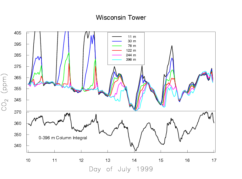
In Wisconsin the local time is lagging UTC by 6 hours. The measurements are made at six height levels on the tower, from 11 m to 396 m above the ground. Near the ground there is a very large diurnal cycle which decreases with altitude. At sunset, when photosynthesis shuts down, the CO₂ mole fraction shoots up, especially at the lowest levels, because plants and soils keep respiring during day and night, releasing CO₂. Sunset occurs at around 1 am UTC, which equals 7 pm local time of the previous day at the tower. During the day photosynthesis is stronger than respiration, causing net removal of CO₂ from the atmosphere, and the CO₂ gradient along the height of the tower reverses. Now the 11 m level near the ground has the lowest CO₂ mole fraction. The mole fraction differences between the levels are very small during the day because the air is vigorously mixed, typically up to altitudes of 1-2 km. During the night the ground cools and the atmosphere becomes stable, with little vertical mixing because the coldest (densest) air is near the ground. The respired CO₂ is trapped in the stable boundary layer near the ground, which may have a thickness of only tens of meters. The buildup of respiratory CO₂ near the ground is more strongly dependent on the atmospheric stability, driven by the weather, than on the rate of respiration. It is more difficult to quantify emissions/removals of CO₂ over the continent than at background sites like Mauna Loa that average over very large areas. Figure 5a also shows slow variations of CO₂ on the time scale of weather systems, several days to a week, with the wind bringing air masses from different directions.

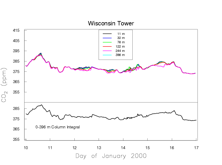
Figure 5b presents one week in January which portrays a typical situation in the winter. There are no strong sources/sinks of CO₂ in the vicinity of the tower, because we see fairly uniform mole fractions along the height of the tower. The variations on the time scale of weather systems remain, due to sources/sinks far away from the tower.

Further reading:

• W.D. Komhyr, T.B. Harris, L.S. Waterman, J.F.S. Chin, and K.W. Thoning, Atmospheric carbon dioxide at Mauna Loa Observatory: 1. NOAA GMCC measurements with a non-dispersive infrared analyzer, Journal of Geophysical Research, vol.94, 8533-8547 (20 June 1989).
• Kirk W. Thoning, Pieter P. Tans, Walter D. Komhyr, Atmospheric carbon dioxide at Mauna Loa Observatory: 2. Analysis of the NOAA GMCC data 1974-1985, Journal of Geophysical Research, vol.94, 8549-8565 (20 June 1989).
• Conglong Zhao and Pieter Tans, Estimating uncertainty of the WMO mole fraction scale for carbon dioxide in air, Journal of Geophysical Research, vol. 111, D08S09, doi: 10.1029/2005JD006003, 2006.
• C. Zhao, P. Tans, and K. Thoning, A high precision manometric system for absolute calibration of CO₂ in dry air, Journal of Geophysical Research, 102, 5885-5894, 1997.