
This is not the latest CarbonTracker update!
Link to latest.
CarbonTracker Documentation
CT2019B release
Nov 12, 2020
Andrew R. Jacobson1,2,
Kenneth N. Schuldt1,2,
John B. Miller2,
Tomohiro Oda3,4,
Pieter Tans2,
Arlyn Andrews2,
John Mund1,2,
Lesley Ott3,
George J. Collatz3,
Tuula Aalto5,
Sara Afshar6,
Ken Aikin7,
Shuji Aoki8,
Francesco Apadula9,
Bianca Baier1,2,
Peter Bergamaschi10,
Andreas Beyersdorf11,
Sebastien C. Biraud12,
Alane Bollenbacher6,
David Bowling13,
Gordon Brailsford14,
James Brice Abshire15,
Gao Chen16,
Huilin Chen17,
Lukasz Chmura18,
Sites Climadat19,
Aurelie Colomb20,
Sébastien Conil21,
Adam Cox6,
Paolo Cristofanelli22,
Emilio Cuevas23,
Roger Curcoll19,
Christopher D. Sloop24,
Ken Davis25,
Stephan De Wekker26,
Marc Delmotte27,
Joshua P. DiGangi16,
Ed Dlugokencky2,
Jim Ehleringer28,
James W. Elkins2,
Lukas Emmenegger29,
Marc L. Fischer12,
Grant Forster30,
Arnoud Frumau31,
Michal Galkowski18,
Luciana V. Gatti32,
Emanuel Gloor33,
Tim Griffis34,
Samuel Hammer35,
László Haszpra36,37,
Juha Hatakka5,
Michal Heliasz38,
Arjan Hensen31,
Ove Hermanssen39,
Eric Hintsa2,
Jutta Holst40,
Dan Jaffe41,
Anna Karion2,
Stephan Randolph Kawa15,
Ralph Keeling6,
Petri Keronen42,
Pasi Kolari42,
Katerina Kominkova43,
Eric Kort44,
Paul Krummel45,
Dagmar Kubistin46,
Casper Labuschagne47,
Ray Langenfelds45,
Olivier Laurent48,
Tuomas Laurila5,
Thomas Lauvaux25,
Bev Law49,
John Lee50,
Irene Lehner38,
Markus Leuenberger51,
Ingeborg Levin35,
Janne Levula42,
John Lin28,
Matthias Lindauer46,
Zoe Loh45,
Morgan Lopez27,
Ingrid T. Luijkx52,53,
Cathrine Lund Myhre39,
Toshinobu Machida54,
Ivan Mammarella55,
Giovanni Manca10,
Alistair Manning56,
Andrew Manning57,
Michal V. Marek43,
Per Marklund58,
Melissa Yang Martin16,
Hidekazu Matsueda59,
Kathryn McKain1,2,
Harro Meijer17,
Frank Meinhardt60,
Natasha Miles25,
Charles E. Miller61,
Meelis Mölder40,
Stephen Montzka2,
Fred Moore2,
Josep-Anton Morgui19,
Shinji Morimoto8,
Bill Munger62,
Jaroslaw Necki18,
Sally Newman63,
Sylvia Nichol14,
Yosuke Niwa54,
Simon O'Doherty64,
Mikaell Ottosson-Löfvenius58,
Bill Paplawsky6,
Jeff Peischl7,
Olli Peltola42,
Jean-Marc Pichon20,
Steve Piper6,
Christian Plass-Dölmer46,
Michel Ramonet27,
Enrique Reyes-Sanchez23,
Scott Richardson25,
Haris Riris15,
Thomas Ryerson7,
Kazuyuki Saito65,
Maryann Sargent62,
Motoki Sasakawa54,
Yousuke Sawa59,
Daniel Say64,
Bert Scheeren17,
Martina Schmidt27,
Andres Schmidt49,
Marcus Schumacher46,
Paul Shepson66,
Michael Shook16,
Kieran Stanley64,
Martin Steinbacher29,
Britton Stephens67,
Colm Sweeney2,
Kirk Thoning2,
Margaret Torn12,
Jocelyn Turnbull68,1,
Kjetil Tørseth39,
Pim van den Bulk31,
Danielle van Dinther31,
Alex Vermeulen40,
Brian Viner69,
Gabriela Vitkova43,
Stephen Walker6,
Dietmar Weyrauch70,
Steve Wofsy62,
Doug Worthy71,
Dickon Young64 and
Miroslaw Zimnoch18
1CIRES, University of Colorado, Boulder, Colorado, USA
2NOAA Earth System Research Laboratory, Global Monitoring Division, Boulder, Colorado, USA
3Global Modeling and Assimilation Office, NASA Goddard Space Flight Center, Greenbelt, Maryland, USA
4Universities Space Research Association, Columbia, Maryland, USA
5Finnish Meteorological Institute, Climate System Research, Helsinki, Finland
6Scripps Institution of Oceanography, University of California, La Jolla, California, USA
7NOAA Earth System Research Laboratory, Chemical Sciences Division, Boulder, Colorado, USA
8Tohoku University, Sendai, Japan
9Ricerca sul Sistema Energetico, Milano, Italy
10European Commission, Joint Research Centre, Ispra, Italy
11California State University, San Bernardino, California, USA
12Lawrence Berkeley National Laboratory, Berkeley, California, USA
13School of Biological Sciences, University of Utah, Salt Lake City, Utah, USA
14National Institute of Water and Atmospheric Research, Wellington, New Zealand
15NASA Goddard Space Flight Center, Greenbelt, Maryland, USA
16NASA Langley Research Center, Hampton, Virginia, USA
17Centre for Isotope Research, University of Groningen, Groningen, Netherlands
18University of Science and Technology (AGH), Krakow, Poland
19Institut de Ciencia i Tecnologia Ambientals, Universitat Autonoma de Barcelona, Barcelona, Spain
20Observatoire de Physique du Globe de Clermont Ferrand, Aubiere, France
21Agence Nationale pour la Gestion des Déchets Radioactifs, France
22Institute of Atmospheric Sciences and Climate (CNR-ISAC), Bologna, Italy
23Agencia Estatal Meteorologia, Santa Cruz de Tenerife, Spain
24Earth Networks, Earth Networks, Inc., Germantown, Maryland, USA
25Penn State University, Department of Meteorology, University Park, Pennsylvania, USA
26University of Virginia, Charlottesville, Virginia, USA
27Laboratoire des Sciences du Climat et de l'Environnement, Gif sur Yvette, France
28Department of Atmospheric Sciences, University of Utah, Salt Lake City, Utah, USA
29Empa, Swiss Federal Laboratories for Materials Science and Technology, Laboratory for Air Pollution/Environmental Technology, Duebendorf, Switzerland
30National Centre for Atmospheric Sciences, University of East Anglia, Norwich, Norfolk, United Kingdom
31Netherlands Organisation for Applied Scientific Research (TNO), Petten, The Netherlands
32National Institute for Space Research (INPE), Sao Paulo, Brazil
33University of Leeds,School of Geography, Leeds, United Kingdom
34University of Minnesota,Department of Soil, Water, and Climate, St. Paul, Minnesota, USA
35Universität Heidelberg, Institut für Umweltphysik, Heidelberg, Germany
36Research Centre for Astronomy and Earth Sciences, Sopron, Hungary
37Hungarian Meteorological Service, Budapest, Hungary
38Lund University, Centre for Environmental and Climate Research, Lund, Sweden
39NILU - Norwegian Institute for Air Research, Kjeller, Norway
40Lund University, Dept. Phys. Geography and Ecosystem Science, Lund, Sweden
41University of Washington, Seattle, Washington, USA
42University of Helsinki, Helsinki, Finland
43CzechGlobe Global Change Research Institute CAS, Brno, Czech Republic
44University of Michigan, Ann Arbor, Michigan, USA
45Commonwealth Scientific and Industrial Research Organization, Oceans and Atmosphere, Aspendale, Victoria, Australia
46Hohenpeissenberg Meteorological Observatory, Hohenpeissenberg, Germany
47South African Weather Service,Cape Point, South Africa
48ICOS Atmospheric Thematic Center, France
49Oregon State University, Corvallis, Oregon, USA
50University of Maine, Orono, Maine, USA
51Climate and Environmental Physics, University of Bern, Bern, Switzerland
52Wageningen University, Wageningen, Netherlands
53 ICOS Carbon Portal, Lund University, Lund, Sweden
54National Instiute for Environmental Studies, Tsukuba, Japan
55Institute for Atmospheric and Earth System Research/Physics, Faculty of Sciences, University of Helsinki, Finland
56Met Office Exeter, Devon , United Kingdom
57Centre for Ocean and Atmospheric Sciences, University of East Anglia, Norfolk, United Kingdom
58Unit for Field-based Forest Research, Swedish University of Agricultural Sciences, Vindeln, Sweden
59Meteorological Research Institute, Tsukuba, Japan
60Umweltbundesamt, Oberried-Hofsgrund, Germany
61Jet Propulsion Laboratory, California Institute of Technology, Pasadena California, USA
62Harvard University, Department of Earth and Planetary Science, Cambridge, Massachusetts, USA
63California Institute of Technology, Pasadena, California, USA
64University of Bristol, Bristol, United Kingdom
65Japan Meteorological Agency, Tokyo, Japan
66Purdue University, West Lafayette, Indiana, USA
67National Center for Atmospheric Research, Boulder, Colorado, USA
68GNS Science,National Isotope Centre, Lower Hutt, New Zealand
69Savannah River National Laboratory, Aikin, South Carolina, USA
70Hohenpeissenberg Meteorological Observatory, Germany
71Environment and Climate Change Canado, Ontario, Canada
Contents
1 Introduction1.1 A tool for science, and policy
1.2 A community effort
1.3 The role of other atmospheric species in constraining the atmospheric carbon budget
1.4 Updates
1.5 Citation and usage policy
1.5.1 Usage Policy
1.5.2 Citing our results
2 Terrestrial biosphere module
2.1 CASA model
2.2 Temporal downscaling
2.2.1 Smooth month-to-month variations
2.3 GFED4.1s and GFED_CMS
3 Fire module
3.1 Global Fire Emissions Database (GFED)
3.2 GFED_CMS: Fluxes from the NASA Carbon Monitoring System
4 Fossil fuel module
4.1 The "Miller" emissions dataset
4.2 The "ODIAC" emissions dataset
4.3 Uncertainties
5 Oceans module
5.1 Air-sea gas exchange
5.2 OIF: the Ocean Inversion Fluxes prior
5.3 pCO2-Clim: Takahashi climatology prior
5.4 Gas-transfer velocity and ocean surface properties
5.5 Specifics of the inversion methodology related to air-sea CO2 fluxes
6 Atmospheric transport
6.1 TM5 offline tracer transport model
6.2 Convective flux fix
7 Observations
7.1 The CarbonTracker observational network
7.2 Adaptive model-data mismatch
7.3 Statistical performance of CT2019B
8 Ensemble data assimilation
8.1 Parameterization of unknowns
8.1.1 Optimization regions
8.1.2 Assimilation window
8.1.3 Ensemble size and localization
8.1.4 Dynamical model
8.2 Covariance structure
8.3 Multiple prior models
8.3.1 Posterior uncertainties in CarbonTracker
9 Ecoregions in CarbonTracker
9.1 What are ecoregions?
9.2 Why use ecoregions?
9.3 Ecosystems within Transcom regions
10 Resources and References
1 Introduction
The goal of the CarbonTracker program is to produce quantitative estimates of atmospheric carbon uptake and release at the Earth's surface that are consistent with observed patterns of CO2 in the atmosphere. CarbonTracker is an inverse model of atmospheric CO2, which means that it attempts to model atmospheric CO2 measurements by adjusting inputs and removals of CO2 at the Earth surface until they best agree with those observational constraints. CarbonTracker is updated on a approximately-annual basis. The current release, CT2019B, provides results from 2000 through the end of 2018. A "near-real" time model product, CT-NRT, extends these results through 2019 and later.1.1 A tool for science, and policy
CarbonTracker is made possible by the long-term monitoring of atmospheric CO2 conducted by many academic and governmental programs around the world (see Sec. 7). These data help improve our understanding of how the land and ocean are responding to Earth's changing climate. The uptake and release of CO2 by these ecosystems is changing due to chemical and physical responses to increased atmospheric CO2 concentrations, to human management of lands and oceans, and to changes in temperature, precipitation, and winds. CarbonTracker is a completely open product. All results, including graphics and tabular data, may be freely used without restriction, although we do request the favor of appropriate acknowledgment (see Sec. 1.5 and https://www.esrl.noaa.gov/ccgg/carbontracker/citation.php). The unrestricted access to all CarbonTracker results means that anyone can scrutinize our work, suggest improvements, and profit from our efforts. We hope this scrutiny will help guide further development of our methods, and improve our ability to monitor, diagnose, and possibly predict the behavior of the global carbon cycle. CarbonTracker also can be relevant for helping to inform carbon policy. Its ability to accurately quantify natural and anthropogenic emissions and uptake at regional scales is currently limited by a sparse observational network. With enough observations however, CarbonTracker and systems like it will be able to monitor regional emissions, including those from fossil fuel use. This will provide an independent check on emissions accounting, including estimates of fossil fuel use based on economic inventories. It can thus provide feedback to policies aimed at limiting greenhouse gas emissions. This independent evaluation of the effectiveness of carbon policy is the bottom line in any mitigation strategy. It has the added advantage of being a constraint provided by the atmosphere itself, where CO2 levels matter most.1.2 A community effort
CarbonTracker is intended to be a tool for the community, and we welcome feedback and collaboration from anyone interested. Our ability to accurately track carbon with more spatial and temporal detail is fundamentally dependent on our collective ability to make enough measurements to characterize variability present in the atmosphere. For example, estimates suggest that observations from tall communication towers (taller than 200m) can tell us about carbon uptake and emission over a radius of only several hundred kilometers. The shows how sparse the current network is. One way to join this effort is by contributing measurements. Regular air samples collected from the surface, towers or aircraft are needed. It would also be very fruitful to expand use of continuous measurements like the ones now being made on very tall (more than 200m) communications towers. Another way to join this effort is by volunteering flux estimates from your own work, to be run through CarbonTracker and assessed against atmospheric CO2 measurements. We also encourage collaborations focused on use of the CarbonTracker model as a tool for scientific analysis. Please contact us if you would like to get involved and collaborate with us.1.3 The role of other atmospheric species in constraining the atmospheric carbon budget
Many laboratories making high accuracy CO2 observations also make many other measurements of the same air, typically other greenhouse gases such as methane (CH4), nitrous oxide (N2O), sulfur hexafluoride (SF6), as well as carbon monoxide (CO) and isotopic ratios of CO2 and CH4. These measurements are usually made as mole fractions, for reasons explained here. These trace gases are relevant for the study of climate change and interesting in their own right, but the additional measurements can also help in identifying sources and sinks of carbon or in understanding carbon cycle processes. For this reason, many air samples are now analyzed for a suite of halocompounds and hydrocarbons. Several of these species can be useful for monitoring air quality, but they can also help with better source apportionment of the greenhouse gases. In addition, the estimation of the source strengths of a number of pollutants could be greatly improved if we were able to quantify fossil fuel CO2 emissions from air measurements for specified regions. The best tracer for quantifying the component of atmospheric CO2 that has been recently added to an air mass through the burning of fossil fuels is the decrease of the carbon-14 (14C) content of CO2. Cosmic rays produce 14C, a radioactive form of carbon, in the higher regions of the atmosphere. It is present in the atmosphere and oceans and in all living organisms and their remains, but coal, oil, and natural gas contain no 14C because it has long decayed away. Currently, 14CO2 measurements are made on only a small subset of the air samples because of higher analysis costs. None of these other data and their relationships have been used directly in this release of CarbonTracker. We expect them to be incorporated gradually at later stages. CarbonTracker is a NOAA contribution to the North American Carbon Program.1.4 Updates
CarbonTracker is updated about once per year to include new data and model improvements. CT2019B provides results from 2000 through 2018, the most recent complete year of observations. Previous versions of CarbonTracker and our CT-NRT (CarbonTracker Near-Real Time) releases are available at the CarbonTracker website. Important revisions of our methods for CT2019B include the following:- Correction of a minor bug in CT2019
- Extension through the end of 2018.
- Revision of fossil fuel emissions to include 2018 increase of about 2%
- Use of reduced prior covariance scaling based on L-curve analysis
- New land and wildfire priors
- Cross-evaluation using withheld assimilation data
- Revised model-data mismatch errors on GLOBALVIEW+ measurements
1.5 Citation and usage policy
1.5.1 Usage Policy
CarbonTracker is an open product of NOAA's Earth System Research Laboratory using data from the NOAA ESRL greenhouse gas observational network and collaborating institutions. Results, including figures and tabular material found on the CarbonTracker website may be used for non-commercial purposes without restriction. We kindly ask you to acknowledge, cite, and/or reference CarbonTracker as described below.1.5.2 Citing our results
- We ask that scientific work that relies heavily on CarbonTracker products is discussed with us before publication, to ensure proper representation of our work and co-authorship if appropriate.
- Please cite as Jacobson et al. (2020)
- The DOI for CT2019B and all its associated products and results is http://dx.doi.org/10.25925/20201008.
- Please use "CT2019B" as the shorthand to refer to our product, not "CT". This identifies both the product and the release version. It is vital to identify the version of the product you are using.
- Note that the product is called "CarbonTracker" without a space character, not "Carbon ␣ Tracker".
- Please include our suggested acknowledgment text in your acknowledgments section.
- Boilerplate model description text provided upon request.
2 Terrestrial biosphere module
The biospheric component of the terrestrial carbon cycle consists of all the carbon stored in `biomass' around us. This includes trees, shrubs, grasses, carbon within soils, dead wood, and leaf litter. Such reservoirs of carbon can exchange CO2 with the atmosphere. Exchange starts when plants take up CO2 during their growing season through the process called photosynthesis (uptake). Most of this carbon is released back to the atmosphere throughout the year through the process of respiration (release). This includes both the decay of dead wood and litter and the metabolic respiration of living plants. Of course, plants can also return carbon to the atmosphere when they burn, as described in Section 3. Even though the yearly sum of uptake and release of carbon amounts to a relatively small number, a few petagrams (one Pg=1015 g)) of carbon per year), the flow of carbon each way is as large as 120 PgC each year. This is why the net result of these flows needs to be monitored in a system such as ours. It is also the reason we need a good physical description (model) of these flows of carbon. After all, from the atmospheric measurements of CO2 we can only see the relatively small net sum of the much larger two-way streams (gross fluxes). Information on what the biospheric fluxes are doing in each season, and in every location on Earth is derived from specialized biosphere models, and fed into our system as a first guess, to be refined by our assimilation procedure.2.1 CASA model
Two biosphere models currently provide first-guess terrestrial fluxes for CT2019B. Both models are versions of the Carnegie-Ames Stanford Approach (CASA) biogeochemical model introduced by Potter et al. (1993). CASA calculates global carbon fluxes using input from weather models to drive biophysical processes, and satellite observed Normalized Difference Vegetation Index (NDVI) to track plant phenology. The models are driven by year-specific weather and satellite observations, and include the effects of fires on photosynthesis and respiration (van der Werf et al., 2003), (van der Werf et al., 2006), (Giglio et al., 2006). Both simulations provide 0.5°×0.5° global fluxes with a monthly time resolution. CASA models directly simulate monthly-mean Net Primary Production (NPP) and heteotrophic respiration (RH) for each terrestrial grid cell being simulated. NPP is the difference in photosynthetic carbon uptake (Gross Primary Production, GPP) and the carbon release by the same plants due to "maintenance respiration", which is also called autotrophic respiration, RA. The carbon uptake represented by NPP and carbon release represented by RH can be differenced to provide Net Ecosystem Exchange (NEE) of CO2. Throughout this discussion, we use the convention that fluxes carry algebraic signs and we adopt the "atmospheric perspective" for those signs. Thus carbon uptake by the terrestrial biosphere is a negative flux to the atmosphere, and release of CO2 back to the atmosphere is a positive flux. This means that we represent all respiration fluxes as positive and GPP as negative, so NEE = NPP + RH. This stands in contrast to convention in the terrestrial carbon community, where all fluxes are generally non-negative.2.2 Temporal downscaling
Use of monthly-mean terrestrial fluxes to simulate atmospheric CO2 is not sufficient to resolve the variability observed at measurement sites. Instead, higher-frequency variations, including the diurnal cycle and effects of passing weather systems must be imposed on the CASA monthly fluxes. Following the logic laid out by Olsen and Randerson (2004), we transform the CASA-supplied monthly-mean NPP and RH fluxes into GPP and total ecosystem respiration, RE = RA + RH. To estimate sub-monthly variations, including diurnal and synoptic variability, the Olsen and Randerson (2004) strategy is to model GPP as a linear function of incoming surface solar radiation and total ecosystem respiration as a function of near-surface temperature. The fundamental assumption needed to apply this scheme is that we can resolve CASA-simulated NPP into GPP and RA. We apply the assumption that GPP is twice NPP, which further implies that RA is the same size as NPP (but of opposite sign):
| (1) |
| (2) |
| (3) |
| (4) |
| (5) |
| (6) |
| (7) |
2.2.1 Smooth month-to-month variations
While the scheme outlined above imposes realistic diurnal- and synoptic-scale variations on monthly-mean GPP and RE, it still allows for abrupt changes from one month to the next. For CT2019B, we add a further processing step designed to remove such unrealistic step changes. We fit smooth curves to the monthly GPP and RE using the piecewise integral quadratic splines (PIQS) of Rasmussen (1991). These PIQS fits are continuous in the first and second derivatives, and have the property of preserving monthly mean flux. We use a similar scheme to smooth over year-to-year step changes in fossil fuel emissions. The final smoothed GPP is
| (8) |
| (9) |
| (10) |
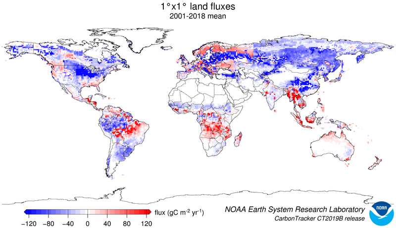
Figure 1: Map of optimized global biosphere fluxes. The pattern of
net ecosystem exchange (NEE) of CO2 of the land biosphere averaged over
the time period indicated, as estimated by CarbonTracker. This NEE
represents land-to-atmosphere carbon exchange from photosynthesis and
respiration in terrestrial ecosystems, and a contribution from fires. It
does not include fossil fuel emissions. Negative fluxes (blue colors)
represent CO2 uptake by the land biosphere, whereas positive fluxes (red
colors) indicate regions in which the land biosphere is a net source of
CO2 to the atmosphere. Units are gC m−2 yr−1.
2.3 GFED4.1s and GFED_CMS
CarbonTracker uses fluxes from CASA runs from two models associated with the GFED project as its first guess for terrestrial biosphere fluxes. We have found a significantly better match to observations when using this output compared to the fluxes from a neutral biosphere simulation. Both of the CASA simulations used in CT2019B (GFED 4.1s and GFED_CMS) are driven by AVHRR NDVI. This satellite driver tends to produce a larger-amplitude annual cycle of NEE compared to the alternative driver, MODIS fPAR. As one of the robust results of atmospheric invrsions is a deeper annual cycle of terrestrial NEE, inversions using NDVI-driven first-guess fluxes perform slightly better than those with a MODIS fPAR driver. The record of atmospheric CO2 calls for a deeper terrestrial biosphere sink than that generally simulated by terrestrial biosphere models like CASA. Inverse models manifesting such a sink generally simulate a larger annual cycle of terrestrial biosphere fluxes, and in particular a deeper boreal summer uptake of carbon dioxide, in the posterior optimized fluxes compared to the prior models (See Fig. 2). We call upon the atmospheric CO2 observations to make this change, and in order to handle these prior model differences the ensemble Kalman filter's prior covariance model has to be appropriately tuned. In short, this prior uncertainty needs to comfortably span differences among the terrestrial biosphere priors, the fossil fuel emissions estimates, and adjustments to fluxes required to bring model predictions into agreement with observations. CT2019B prior covariances have been adjusted compared to prior releases, and details on this adjustment can be found in Section 8.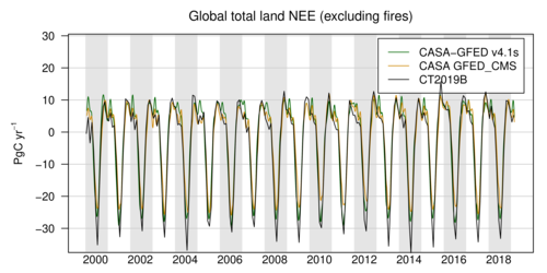
Figure 2: Time series of global-total terrestrial biosphere flux between
the two priors and the CT2019B posterior. Global CO2 uptake by the land
biosphere, expressed in PgC yr−1, excluding emissions by wildfire.
Positive flux represents emission of CO2 to the atmosphere, and the
negative fluxes indicate times when the land biosphere is a sink of CO2.
Optimization against atmospheric CO2 data requires a larger land sink
than in either prior, which effectively requires a deeper annual cycle.
This is shown by the CT2019B posterior (black).
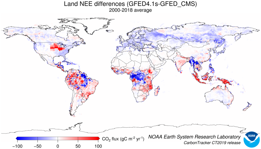
Figure 3: Differences in long-term mean terrestrial biosphere fluxes
between the two priors. Red indicates areas where the GFED4.1s prior has
less terrestrial uptake (or more outgassing to the atmosphere) than the
GFED_CMS prior, and blue represents the opposite. Units are gC m−2 yr−1.
CarbonTracker CT2019B is a full reanalysis of the 2000-2018 period
using new fossil fuel emissions, CASA-GFED v4.1s and GFED_CMS fire
emissions, and first-guess biosphere model fluxes derived from
CASA-GFED v4.1s for the first of our inversions, and from CASA GFED_CMS for
the second inversion.
Due to the inclusion of fires, inter-annual variability in weather and
NDVI, the fluxes for North America start with a small net
flux even before optimizing the fluxes. This first-guess flux ranges
from neutral exchange to about 0.5 PgC yr−1 of uptake.
3 Fire module
Vegetation fires are an important part of the carbon cycle and have been so for many millennia. Even before human civilization began to use fires to clear land for agricultural purposes, most ecosystems were subject to natural wildfires that would rejuvenate old forests and bring important minerals to the soils. When fires consume part of the landscape in either controlled or natural burning, carbon dioxide (amongst many other gases and aerosols) is released in large quantities. Each year, vegetation fires emit around 2 PgC as CO2 into the atmosphere, mostly in the tropics. Currently, a large fraction of wildfire is started by humans. This is mostly intentional to clear land for agriculture, or to re-fertilize soils before a new growing season. This important component of the carbon cycle is monitored mostly from space, while sophisticated `biomass burning' models are used to estimate the amount of CO2 emitted by each fire. Such estimates are then used in CarbonTracker to prescribe the emissions. These emissions are not modified in the optimization (inverse modeling) process. In CT2019B we use two fire emissions datasets, each with at least daily temporal resolution. The GFED4.1s emissions are modeled at 3-hourly intervals, and GFED_CMS emissions are available at daily resolution.3.1 Global Fire Emissions Database (GFED)
CT2019B uses GFED4.1s (Giglio et al., 2013), (van der Werf et al., 2017) as one of the fire modules to estimate biomass burning. GFED4.1s is a variant of the CASA biogeochemical model as described in the terrestrial biosphere model documentation to estimate the carbon fuel in various biomass pools. The dataset consists of 1° × 1° gridded monthly burned area, fuel loads, combustion completeness, and fire emissions (Carbon, CO2, CO, CH4, NMHC, H2, NOx, N2O, PM2.5, Total Particulate Matter, Total Carbon, Organic Carbon, Black Carbon) for the time period spanning January 1997 - December 2018, of which we currently only use CO2. The GFED burned area is based on MODIS satellite observations of fire counts. These, together with detailed vegetation cover information and a set of vegetation specific scaling factors, allow predictions of burned area over the time span that active fire counts from MODIS are available. The relationship between fire counts and burned area is derived, for the specific vegetation types, from a `calibration' subset of 500m resolution burned area from MODIS in the period 2001-2004. Once burned area has been estimated globally, emissions of trace gases are calculated using the CASA biosphere model. The seasonally changing vegetation and soil biomass stocks in the CASA model are combusted based on the burned area estimate, and converted to atmospheric trace gases using estimates of fuel loads, combustion completeness, and burning efficiency. For CT2019B, we also apply temporal scaling factors updated from Mu et al. (2011) to downscale the GFED4.1s CO2 emissions from monthly averages to emissions with 3-hourly resolution.3.2 GFED_CMS: Fluxes from the NASA Carbon Monitoring System
The NASA GFED_CMS team uses a variant of the GFED4 system to produce alternative fire emissions. This model uses GIMSS NDVI, the GFEDv3 fire model and GFEDv4 burned area. Fire emissions are available on a daily basis from 2003-2017. For 2000-2002, and for 2018-2019, we apply the climatology of GFED_CMS fire emissions, computed from its 2003-2017 mean. Note that the GFED_CMS team produces temporally-downscaled GPP, heterotrophic respiration, and fires with 3-hourly resolution. This is done using MERRA meteorology using a scheme similar to Olsen and Randerson (2004). We do not use this downscaled product, in part because the MERRA meteorology is different from the ECMWF meteorology, and in part because the spatial resolution of the MERRA meteorology is different from our 1° × 1° flux grid. This means that we are limited to daily resolution of GFED_CMS fire emissions: unlike the GFED4.1s fire emissions, these have no diurnal cycle.4 Fossil fuel module
Human beings first influenced the carbon cycle through land-use change. Early humans used fire to control animals and later cleared forests for agriculture. Over the last two centuries, following the industrial and technical revolutions and continuing global population increase, fossil fuel combustion has become the largest anthropogenic source of CO2. Coal, oil and natural gas combustion are the most common energy sources in both developed and developing countries. Important sectors of the economy-power generation, transportation, residential & commercial building heating, and industrial processes-rely on fossil fuels. The continued growth of fossil fuel combustion has led to a steady increase of global CO2 emissions to the atmosphere (Fig. 4). According to the Carbon Dioxide Information and Analysis Center (CDIAC) as reported in Boden et al. (2017), world emissions of CO2 from fossil fuel burning, cement manufacturing, and flaring reached 5 billion metric tons of carbon per year (PgC yr−1) in the decade of the 1970s. Estimates extrapolated by the CarbonTracker team indicate that global total emissions exceeded 10 PgC yr−1 for the first time in 2018. One petagram of carbon, PgC, is equal to 1015 grams of carbon, or one billion metric tons of carbon. To convert to mass of CO2 emitted, one would multiply by the factor [44/12], representing the molecular weight of CO2 compared to the atomic weight of carbon.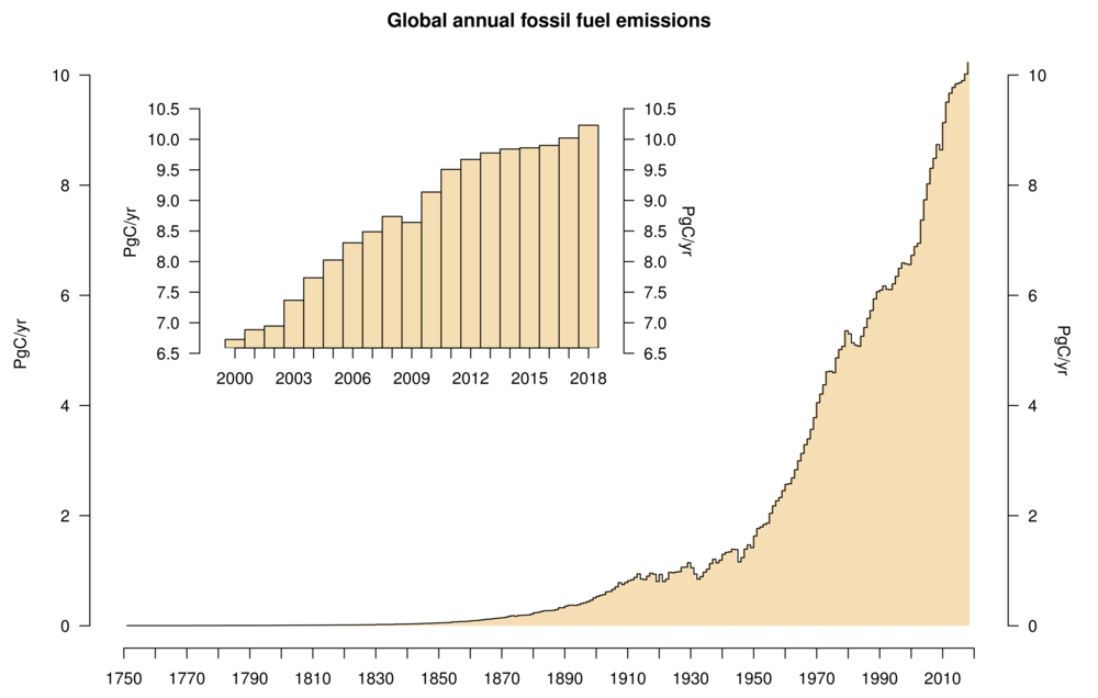
Figure 4: Time series of annual global fossil fuel emissions, in units
of PgC yr−1 (billion metric tons of C per year). Values from 1751 to
2014 are from
Boden et al. (2017), and later values are extrapolated
using consumption growth rate data of
British Petroleum (2019). Inset figure
shows the CT2019B period of analysis, 2000-2018.
U.S. input of CO2 to the atmosphere from fossil fuel
burning in 2015 was 1.4 PgC, representing 14% of the global total.
North American emissions have remained nearly constant since 2000,
with a slight decrease after the economic slowdown of 2008. On the other hand, emissions
from developing economies such as the People's Republic of China have
been increasing. Emissions from China in 2015 were 2.6 PgC yr−1,
representing 27% of the global total.
In most global and regional carbon flux estimation systems,
including CarbonTracker, fossil fuel CO2 emissions are not
optimized. Instead, these emissions are imposed and are not subject to
revision by the inverse modeling framework. Global mass balance requires
that any errors in fossil fuel emissions be compensated by opposing
errors in land and ocean CO2 exchange. Thus it is vital that
fossil fuel CO2 emissions are prescribed accurately, so that flux
estimates for the land biosphere and oceans are robust. The fossil
fuel emissions source data we use are available on an
annually-integrated global and national basis. This aggregate
information needs to be gridded before being incorporated into
CarbonTracker. The major uncertainty in this process is distributing
the national-annual emissions spatially across a nation and temporally
into hourly contributions. In CT2019B, two different fossil fuel
CO2 emissions datasets were used to help assess the uncertainty
in this mapping process. These two emissions products are called the
"Miller" and "ODIAC" emissions datasets. These two datasets have
very similar global and national emissions for each year, but
differ in how those emissions are distributed spatially and
temporally.
Whereas previous CarbonTracker releases used monthly-constant fossil
fuel emissions, in CT2015 we introduced the use of temporal scaling
factors to simulate day-of-week and diurnal variability for those
emissions. These "Temporal Improvements for Modeling Emissions by
Scaling" (TIMES) scaling factors, introduced by
Nassar et al. (2013),
are again applied to both the Miller and ODIAC emissions modules for
CT2019B. The scaling factors consist of seven day-of-week global
scaling factor maps, and 24 hourly global scaling factor maps to
represent the diurnal cycle. For use in TM5, the hourly scaling
factors were aggregated to three-hourly factors to accommodate the
time step of the model.
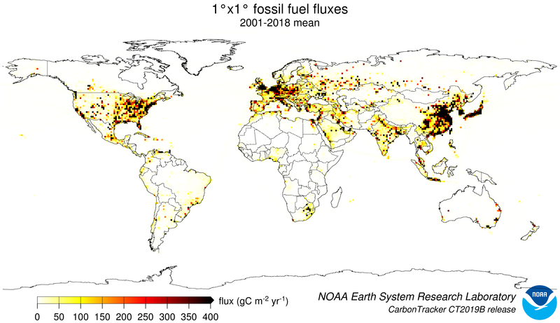
Figure 5: Spatial distribution of fossil fuel emissions. This
is a spatial average of the Miller and ODIAC emissions inventories.
4.1 The "Miller" emissions dataset
- Global Totals The Miller fossil fuel emission inventory is derived from independent global total and spatially-resolved inventories. Annual global total fossil fuel CO2 emissions are from the Carbon Dioxide Information and Analysis Center (Boden et al., 2017) which extend through 2014. In order to estimate these fluxes through 2018, we extrapolate using the percentage increase or decrease for each fuel type (solid, liquid, and gas) in each country from the British Petroleum (2019). To estimate emissions for the first few months of 2019 (required by CarbonTracker's 12-week assimilation window), no increase is applied to 2018 values (British Petroleum, 2019).
- Spatial Distribution Miller fossil-fuel CO2 fluxes are spatially distributed in two steps: First, the coarse-scale country totals through 2014 from Boden et al. (2017) are mapped onto a 1° × 1° grid according to the spatial patterns from the EDGAR v4.2 inventories (European Commission, 2011). The spatial pattern varies by year up until the end of the EDGAR v4.2 product in 2008. After this, the trends estimated in each pixel are linearly extrapolated. Note that while EDGAR provides annual emissions estimates at 1° × 1° resolution, their totals do not agree with those from CDIAC (Boden et al., 2017). Thus, only the spatial patterns in EDGAR are used. The CDIAC country-by-country totals sum to about 95% of the global total emissions; the remaining 5% is mapped to global shipping routes according to EDGAR, which we treat as a proxy for bunker fuel emissions.
- Temporal Distribution For North America between 30 and 60°N, the Miller system imposes a seasonal cycle derived from the first and second harmonics (Thoning et al., 1989) of the Blasing et al. (2004) analysis for the United States. The Blasing analysis has 10% higher emissions in winter than in summer. This scheme defines a fixed fraction of emissions for each month, so while the shape of the annual cycle is invariant, the amplitude of that cycle scales with the annual total emissions. For Eurasia, a set of seasonal emissions factors from EDGAR distributed by emissions sector is used to define fossil fuel seasonality. As in North America, this seasonality is imposed only from 30-60°N. The Eurasian seasonal amplitude is about 25%, significantly larger than that in North America, owing to the absence of a secondary summertime maximum due to air conditioning. See Figure 6 for the resulting time series of fossil fuel emissions. In order to avoid discontinuities in the fossil fuel emissions between consecutive years, a spline curve that conserves annual totals (Rasmussen, 1991) is fit to seasonal emissions in each 1° × 1° grid cell.
4.2 The "ODIAC" emissions dataset
- Global Totals We use the ODIAC2018 fossil fuel emission inventory (Oda et al., 2018), (Oda and Maksyutov, 2011), (Oda and Maksyutov, 2015) as one of our fossil fuel emissions estimates. ODIAC is also derived from independent global and country emission estimates from CDIAC, but national emission estimates used were taken from the year 2018 edition of CDIAC estimates (Boden et al., 2018). Differences between the Boden et al. (2018) global total and country-by-country totals were ascribed to the entire emissions field. Annual country total fossil fuel CO2 emissions for 2014-2017 were extrapolated using the BP Statistical Review of World Energy (British Petroleum, 2019). Emissions for 2018 were estimated by applying a global scaling factor representing the reported ∼ 2.1% increase compared to 2017 emissions (British Petroleum, 2019). Emissions for 2019 were set to those of 2018.
- Spatial Distribution ODIAC emissions are spatially distributed using many available "proxy data" that explain spatial extent of emissions according to emission types (emissions over land, gas flaring, aviation and marine bunker). Emissions over land were distributed in two steps: First, emissions attributable to power plants were mapped using geographical locations (latitude and longitude) provided by the global power plant dataset CARbon Monitoring and Action, CARMA. Next, the remaining land emissions (i.e. land total minus power plant emissions) were distributed using nightlight imagery collected by U.S. Air Force Defense Meteorological Satellite Project (DMSP) satellites. Emissions from gas flaring were also mapped using nightlight imagery. Emissions from aviation were mapped using flight tracks adopted from UK AERO2k air emission inventory. It should be noted that currently, air traffic emissions are emitted at ground level within CarbonTracker. Emissions from marine bunker fuels are placed entirely in the ocean basins along shipping routes according to patterns from the EDGAR database.
- Temporal Distribution The CDIAC estimates used for mapping emissions in ODIAC only describe how much CO2 was emitted in a given year. To present seasonal changes in emissions, we used the CDIAC 1° × 1° monthly fossil fuel emission inventory (Andres et al., 2011). The CDIAC monthly data utilizes the top 20 emitting countries' fuel (coal, oil and gas) consumption statistics available to estimate seasonal change in emissions. Monthly emission numbers at each pixel were divided by annual total and then a fraction to annual total was obtained. Monthly emissions in the ODIAC inventory were derived by multiplying this fraction by the emission in each grid cell.
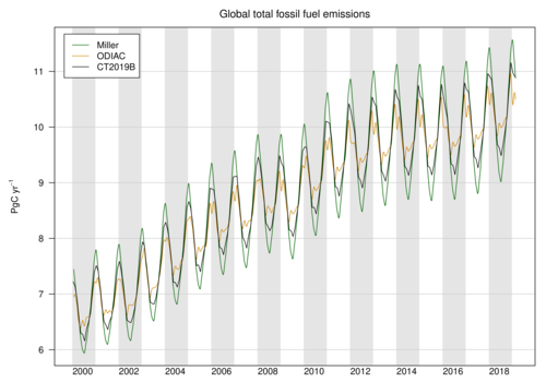
Figure 6: Time series of global fossil fuel emissions showing annual cycles. The Miller (green)
and ODIAC (tan) estimates are each used by half of the sixteen inversions
in the CT2019B suite, so the CT2019B (black) inventory is effectively an
average of Miller and ODIAC. Note that fossil fuel emissions are not
optimized in CarbonTracker.
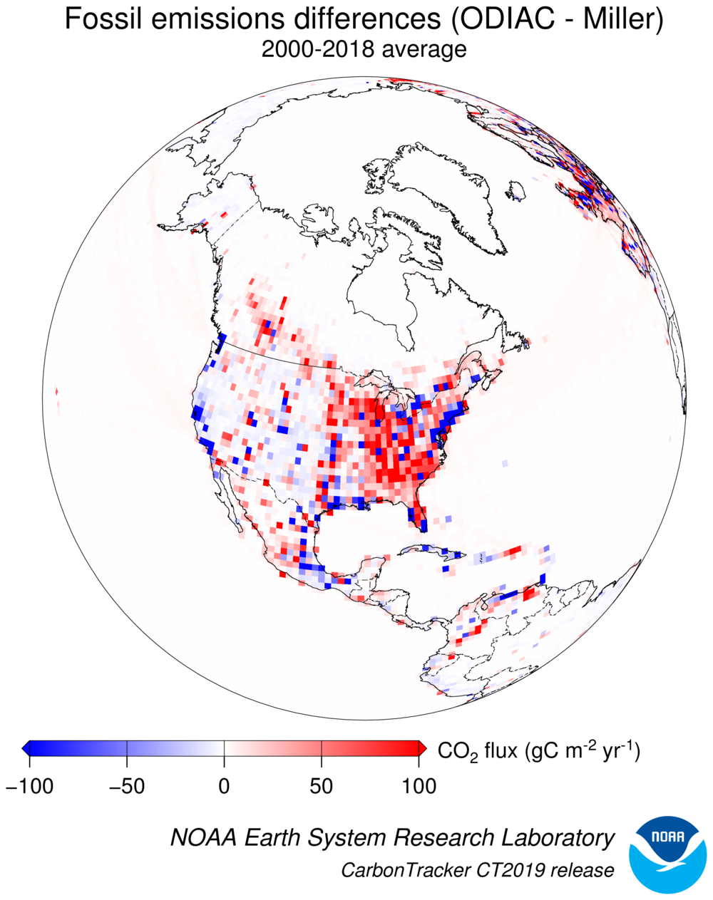
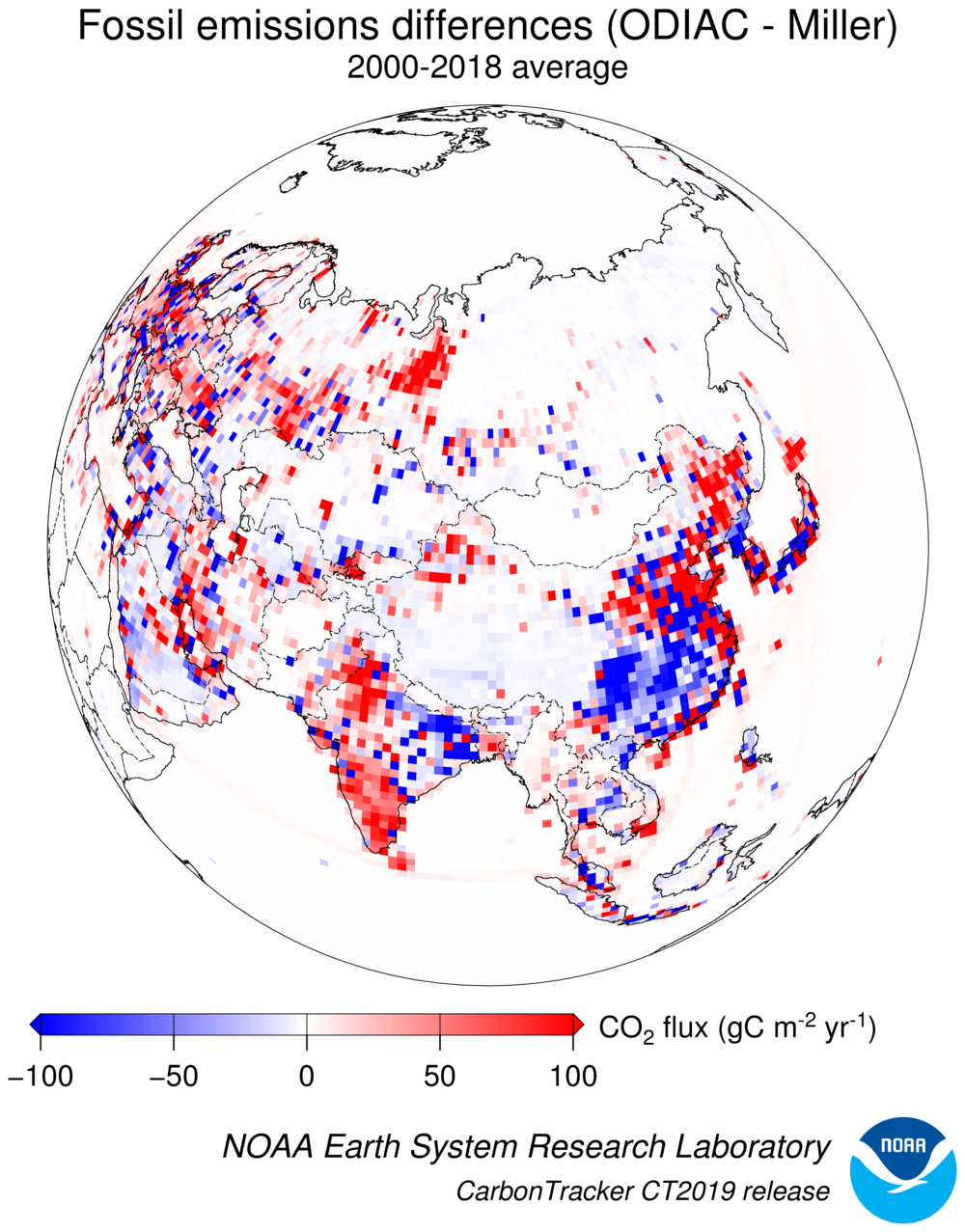
Figure 7: Spatial differences in long-term mean fossil fuel emissions
between the two priors. Note that both the Miller and ODIAC emissions
inventories use the same country totals, but have different models for
spatial distribution of that flux within countries.
4.3 Uncertainties
Marland (2008) attached an uncertainty of about 5% (95% confidence interval; approximately 2-σ) to the global total fossil fuel source. Recent estimates by Andres et al. (2014) put a larger uncertainty of 8.4% (2-σ) on the CDIAC global total. Uncertainties for individual regions of the world, and for sub-annual time periods are likely to be larger. Additional uncertainties are introduced when the emissions are distributed in space and time. In the Miller dataset, the overall Eurasian seasonality is based on scaling factors derived only from Western Europe and thus highly uncertain, but most likely a better representation than assuming no emission seasonality at all. Similarly, the use of the CDIAC monthly emission dataset for modeling seasonality introduces additional uncertainty in ODIAC. The additional uncertainty for the global total in the monthly CDIAC emission, which is solely due to the method for estimating seasonality, is reported as 6.4% (Andres et al., 2011). As mentioned earlier, fossil fuel emissions are not optimized in the current CarbonTracker system, similar to nearly all carbon data analysis systems. Spatial and temporal atmospheric CO2 gradients arise from terrestrial biosphere and fossil-fuel sources. These gradients, which are interpreted by CarbonTracker, are difficult to attribute to one or the other cause. This is because atmospheric sampling sites have historically been established in locations remote from biospheric and anthropogenic sources, especially in the temperate Northern Hemisphere. Given that surface CO2 flux due to biospheric activity and oceanic exchange is much more uncertain compared to fossil fuel emissions, CarbonTracker, like most current carbon dioxide data assimilation systems, does not attempt to optimize fossil fuel emissions. That is, the contribution of CO2 from fossil fuel burning to observed CO2 mole fractions is considered known. As detailed above, however, in CarbonTracker an effort is made to account for some aspects of fossil fuel uncertainty by using two different fossil fuel estimates. From a technical point of view, extra land biosphere prior flux uncertainty is included in the system to represent the random errors in fossil fuel emissions. Eventually, fossil fuel emissions could be optimized within CarbonTracker, especially with the addition of 14CO2 observations as constraints (Basu et al., 2016).5 Oceans module
The oceans play an important role in the Earth's carbon cycle. They are the largest long-term sink for carbon and have an enormous capacity to store and redistribute CO2 within the Earth system. Oceanographers estimate that about 48% of the CO2 from fossil fuel burning has been absorbed by the ocean (Sabine et al., 2004). The dissolution of CO2 in seawater shifts the balance of the ocean carbonate equilibrium towards a more acidic state with a lower pH. This effect is already measurable (Caldeira and Wickett, 2003), and is expected to become an acute challenge to shell-forming organisms over the coming decades and centuries. Although the oceans as a whole have been a relatively steady net carbon sink, CO2 can also be released from oceans depending on local temperatures, biological activity, wind speeds, and ocean circulation. These processes are all considered in CarbonTracker, since they can have significant effects on the ocean sink. Improved estimates of the air-sea exchange of carbon in turn help us to understand variability of both the atmospheric burden of CO2 and terrestrial carbon exchange.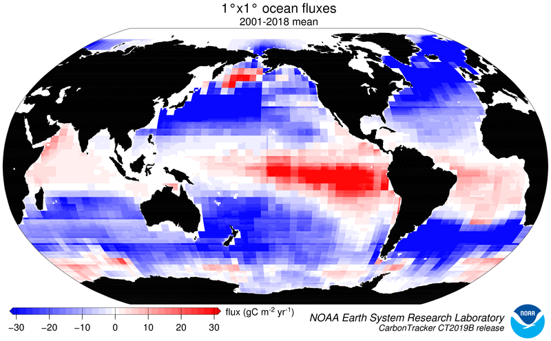
Figure 8: Posterior long-term mean ocean fluxes from
CarbonTracker. The pattern of air-sea exchange of CO2 averaged over the
time period indicated, as estimated by CarbonTracker. Negative fluxes
(blue colors) represent CO2 uptake by the ocean, whereas positive fluxes
(red colors) indicate regions in which the ocean is a net source of CO2
to the atmosphere. Units are gC m−2 yr−1.
The initial release of CarbonTracker (CT2007) used climatogical
estimates of CO2 partial pressure in surface waters (pCO2)
from
Takahashi et al. (2002) to compute a first-guess air-sea flux. This
air-sea pCO2 disequilibrium was modulated by a surface barometric
pressure correction before being multiplied by a gas-transfer
coefficient to yield a flux. Starting with CT2007B and continuing
through the CT2011_oi release, the air-sea pCO2 disequilibrium
was imposed from analysis of ocean inversions
(Jacobson et al., 2007),"OIF" results, with short-term flux variability
derived from the atmospheric model wind speeds via the gas transfer
coefficient. The barometric pressure correction was removed so that
climatological high- and low-pressure cells did not bias the long-term
means of the first guess fluxes.
In CT2019B, two models are used to provide prior estimates of air-sea
CO2 flux. The OIF scheme provides one of these flux priors, and
the other is an updated version of the
Takahashi et al. (2009) pCO2
climatology.
5.1 Air-sea gas exchange
Oceanic uptake of CO2 in CarbonTracker is computed using air-sea differences in partial pressure of CO2 inferred either from ocean inversions (called "OIF" henceforth), or from a compilation of direct measurements of seawater pCO2 (called "pCO2-clim" henceforth). These air-sea partial pressure differences are combined with a gas transfer velocity computed from wind speeds in the atmospheric transport model to compute fluxes of carbon dioxide across the sea surface. In either method, the first-guess fluxes have no interannual variability (IAV) other than a smooth trend. IAV in oceanic CO2 flux is due to anomalies in surface pCO2, such as those that occur in the tropical eastern Pacific during an El Niño, and to associated variability in winds, ocean circulation, and sea-surface properties. In CarbonTracker, only the surface winds (and hence gas transfer), manifest these interannual anomalies; the remaining IAV of flux must be inferred from atmospheric CO2 signals. In the following sections we describe the two ocean flux prior models. We then describe the air-sea gas transfer velocity parameterization and discuss detais of the inversion methodology specific to oceanic exchange of CO2.5.2 OIF: the Ocean Inversion Fluxes prior
For the OIF prior, long-term mean air-sea fluxes and the uncertainties associated with them are derived from the ocean interior inversions reported in Jacobson et al. (2007). These ocean inversion flux estimates are composed of separate preindustrial (natural) and anthropogenic flux inversions based on the methods described in Gloor et al. (2003) and biogeochemical interpretations of Gruber et al. (1996). The uptake of anthropogenic CO2 by the ocean is assumed to increase in proportion to atmospheric CO2 levels, consistent with estimates from ocean carbon models. OIF contemporary pCO2 fields were computed by summing the preindustrial and anthropogenic flux components from inversions using five different configurations of the Princeton/GFDL MOM3 ocean general circulation model (Pacanowski and Gnanadesikan, 1998), then dividing by a gas transfer velocity computed from the European Centre for Medium-Range Weather Forecasts (ECMWF) ERA40 reanalysis. There are two small differences in first-guess fluxes in this computation from those reported in Jacobson et al. (2007). First, the five OIF estimates all used Takahashi et al. (2002) pCO2 estimates to provide high-resolution patterning of flux within inversion regions (the alternative "forward" model patterns were not used). To good approximation, this choice only affects the spatial and temporal distribution of flux within each of the 30 ocean inversion regions, not the magnitude of the estimated flux. Second, wind speed differences between the ERA40 product used in the offline analysis and the ECMWF operational model used in the online CarbonTracker analysis result in small deviations from the OIF estimates. Other than the smooth trend in anthropogenic flux assumed by the OIF results, interannual variability (IAV) in the first guess ocean flux comes entirely from wind speed effects on the gas transfer velocity. This is because the ocean inversions retrieve only a long-term mean and smooth trend.5.3 pCO2-Clim: Takahashi climatology prior
The pCO2-Clim prior is derived from the Takahashi et al. (2009) climatology of seawater pCO2. This climatology was created from about 3 million direct observations of seawater pCO2 around the world between 1970 and 2007. With the exception of measurements in the Bering Sea, these observations were all linearly extrapolated to the corresponding month of the year 2000 by assuming a constant trend of 1.5 μatm yr−1. This set of global monthly measurements corrected to the reference year 2000 was then interpolated onto a regular grid using a modeled surface current field. The Takahashi et al. (2009) product goes beyond providing this estimate of surface water pCO2. They also compute climatological air-sea exchange of CO2 by using the GLOBALVIEW-CO2 atmospheric carbon dioxide product to compute air-sea ∆pCO2, sea surface properties inferred from ocean climatologies, and winds from atmospheric reanalysis to estimate gas-transfer velocity. Unlike many other atmospheric analyses, we have chosen not to use the climatological fluxes as our prior, nor to use the climatological ∆pCO2. Instead, we take only the seawater pCO2 distribution from the Takahashi et al. (2009) climatology-our atmospheric model provides both pCO2 in the air at the sea surface and the winds needed to estimate gas transfer. Seawater pCO2 is extrapolated from 2000 to the actual year of the CarbonTracker simulation using a presumed increase of 1.5 μatm yr−1 at every point in the global ocean. This is the same trend used in Takahashi et al. (2009) to normalize observations from many years to the reference year of the analysis (2000).5.4 Gas-transfer velocity and ocean surface properties
Both priors use CO2 solubilities and Schmidt numbers computed from World Ocean Atlas 2009 (WOA09) climatological fields of sea surface temperature and sea surface salinity fields (Levitus et al., 2010). Gas transfer velocity in CarbonTracker is parameterized as a quadratic function of wind speed following Wanninkhof (1992), using the formulation for instantaneous winds. Gas exchange is computed every 3 hours using wind speeds from the ECMWF operational model as represented by the atmospheric transport model. Air-sea transfer is inhibited by the presence of sea ice, and for this work fluxes are scaled by the daily sea ice fraction in each gridbox provided by the ECMWF forecast data.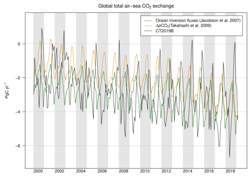
Figure 9: Comparison of air-sea flux priors and the CT2019B
posterior. Global CO2 uptake by the ocean, expressed in
PgC yr−1. Positive flux represents a gain of CO2 to the
atmosphere, and the negative numbers here indicate that the ocean is
a sink of CO2. While both priors manifest similar trends of
increasing oceanic uptake of CO2, the OIF prior (in green) has
more oceanic uptake and a greater annual cycle than the
pCO2-clim prior (in tan). The CT2019B across-model posterior
estimate is shown in black for comparison.
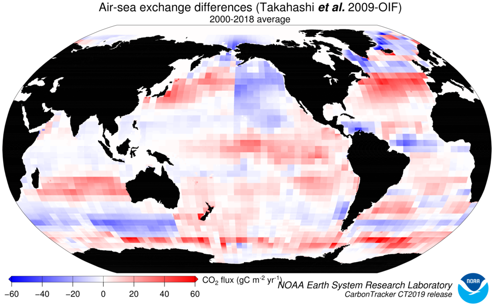
Figure 10: Differences in long-term mean ocean fluxes between the two
priors. Red indicates areas where the pCO2-clim prior has less oceanic
uptake (or more outgassing to the atmosphere) than the OIF prior, and
blue represents the opposite. Units are gC m-2 yr-1.
5.5 Specifics of the inversion methodology related to air-sea CO2 fluxes
The first-guess fluxes described here are subject to scaling during the CarbonTracker optimization process, in which atmospheric CO2 mole fraction observations are combined with transport simulated by the atmospheric model to infer flux signals. Prior air-sea fluxes are adjusted within each of of the 30 ocean inversion regions. In this process, signals of terrestrial flux in atmospheric CO2 distribution can be erroneously interpreted as being caused by oceanic fluxes. This flux "aliasing" or "leakage" is evident in some regions as a change in the shape of the seasonal cycle of air-sea flux. Prior uncertainties for the OIF and pCO2-clim models are specified as uncertainties on scaling factors multiplying net CO2 flux in each of the 30 ocean inversion regions. The pCO2-clim prior has independent regional uncertainties (a diagonal prior covariance matrix), with the uncertainty standard deviation on each region set to 40%. The OIF prior uncertainty has a fully-covariate covariance matrix with off-diagonal elements representing the results of the ocean inversion of Jacobson et al. (2007). The pre-industrial flux uncertainty is time-independent, but the anthropogenic flux uncertainty grows in time as anthropogenic flux uptake increases. The latter is scaled to the simulation date, then added to the former. Total uncertainties are consistent with the Jacobson et al. (2007) results.6 Atmospheric transport
The link between observations of CO2 in the atmosphere and the exchange of CO2 at the Earth's surface is transport in the atmosphere: storm systems, cloud complexes, and weather of all sorts cause winds that transport CO2 around the world. As a result, local surface CO2 exchange events like fires, forest growth, and ocean upwelling can have impacts at remote locations. To simulate the winds and the weather, CarbonTracker uses sophisticated numerical models that are driven by the daily weather forecasts from the specialized meteorological centers of the world. Since CO2 does not decay or react in the lower atmosphere, the influence of emissions and uptake in locations such as North America and Europe are ultimately seen in our measurements even at the South Pole. Getting the transport of CO2 just right is an enormous challenge, and costs us almost all of the computer resources for CarbonTracker. To represent the atmospheric transport, we use the Transport Model 5 (TM5). This is a community-supported model whose development is shared among many scientific groups with different areas of expertise. TM5 is used for many applications other than CarbonTracker, including forecasting air-quality, studying the dispersion of aerosols in the tropics, tracking biomass burning plumes, and predicting pollution levels that future generations might have to deal with.6.1 TM5 offline tracer transport model
TM5 is an offline global chemical transport model with two-way nested grids. In this global model, regions for which high-resolution simulations are desired can be nested in the coarser global grid. The advantage to this approach is that transport simulations can be performed with a regional focus without the need for boundary conditions. Further, this approach allows measurements outside the "zoom" domain to constrain regional fluxes in the data assimilation, and ensures that regional estimates are consistent with global constraints. TM5 is based on a predecessor model TM3, with improvements in the advection scheme, vertical diffusion parameterization, and meteorological preprocessing of the wind fields (Krol et al., 2005). The model is developed and maintained jointly by the Institute for Marine and Atmospheric Research Utrecht (IMAU, The Netherlands), the Joint Research Centre (JRC, Italy), the Royal Netherlands Meteorological Institute (KNMI), the Netherlands Institude for Space Research (SRON), and the NOAA Earth System Research Laboratory (ESRL). In CarbonTracker, TM5 separately simulates advection, deep and shallow convection, and vertical diffusion in both the planetary boundary layer and free troposphere. The carbon dioxide concentrations predicted by CarbonTracker do not feed back onto these predictions of winds. Prior to use in TM5, ECMWF meteorological data are preprocessed into coarser grids, with attention to retrieving a flow that conserves tracer mass. Like most numerical weather prediction models, advection in the parent ECMWF model is not strictly mass-conserving, so this step is crucial. In CarbonTracker, TM5 is currently run at a global 3° longitude × 2° latitude resolution with a nested regional grid over North America at 1° × 1° resolution (Figure 11). TM5 uses a dynamically-variable time step with a maximum length of 90 minutes. This overall timestep is dynamically reduced to maintain numerical stability, generally during times of high wind speeds. The timestep is divided in half and individual advection, diffusion, convection, and chemistry operators are applied symmetrically in each half step. Furthermore, transport operators in nested grids are modeled at shorter timesteps, so processes at the finest scales are conducted at an effective timestep of one-quarter the overall timestep. See Krol et al. (2005) for details.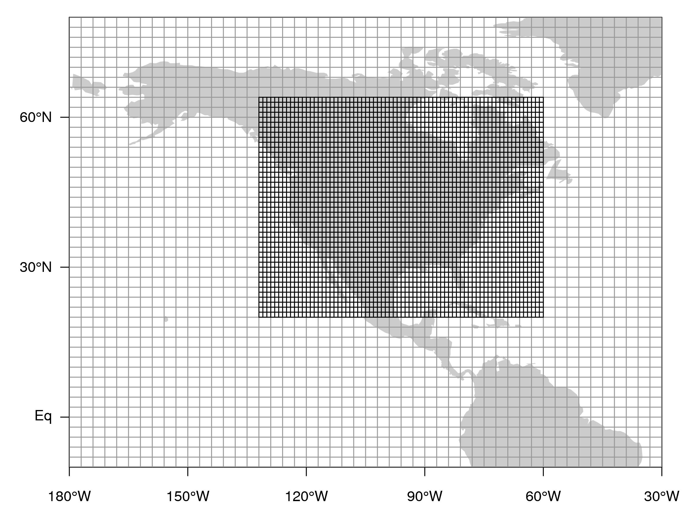
Figure 11: Nested grids used in CarbonTracker over North America. TM5 is
a global model, but it employs nested grids to provide higher
resolution over regions of interest. This figure shows the
1° × 1° nested regional grid over North America and a portion of
the global 3° longitude × 2° latitude grid.
The winds which drive TM5 come from the ERA-interim reanalysis
implemented in the European Centre for
Medium-Range Weather Forecasts (ECMWF) modeling system. The
ERA-Interim reanalysis uses Cy31r2 version of the ECMWF Integrated
Forecast System (IFS) model, which was used for the operational
forecasts up until June 2007. That model uses a 30-minute time step
and a a spectral T255 horizontal resolution, which corresponds to
approximately 79 km spacing on a reduced Gaussian grid. This version
of the IFS has 60 model layers in the vertical, of which TM5 uses a
25-layer subset. These levels are listed in Table 1.
| Model Level | Mean Height (m) | Model Level | Mean Height (m) |
| 1 | 25 | 14 | 9114 |
| 2 | 103 | 15 | 10588 |
| 3 | 247 | 16 | 12184 |
| 4 | 480 | 17 | 13928 |
| 5 | 814 | 18 | 15843 |
| 6 | 1259 | 19 | 17983 |
| 7 | 1822 | 20 | 20412 |
| 8 | 2508 | 21 | 24433 |
| 9 | 3317 | 22 | 30003 |
| 10 | 4248 | 23 | 35895 |
| 11 | 5300 | 24 | 43210 |
| 12 | 6467 | 25 | 123622 |
| 13 | 7741 |
Table 1: Mean mid-level heights above ground in meters for the TM5
model using ERA-interim transport.
6.2 Convective flux fix
Until recently, TM5 was known to have difficulties representing the global surface distribution of sulfur hexafluoride (SF6, see Figure 12 and Peters et al. (2004). SF6 is a nearly inert tracer in the atmosphere, with very small surface and atmospheric sinks and an atmospheric lifetime of about 1,000 years. Consequently, its global budget is very well known from observations alone. It is thought to be released mainly via leakage from electrical transformers. Since the electrical distribution system is closely tied to fossil fuel consumption, SF6 is often considered an analog for fossil fuel CO2 in the atmosphere. It is useful for understanding the rate at which Northern Hemisphere land surfaces are ventilated to the free troposphere, and the rate of interhemispheric exchange in models (Patra et al., 2011). As a result of more than a decade's worth of work on understanding the apparently sluggish mixing in TM5 as revealed by SF6 simulations, a fault in one of the vertical mixing parameterizations of the model was discovered. When it was originally created, TM5 implemented the same planetary boundary layer (PBL) mixing and convection schemes as the parent ECMWF model. Recent comparisons between TM5, the ECMWF parent model, and radiosonde profile data show that the PBL scheme in TM5 performs similarly to that of the parent ECMWF model. The convective scheme, however, does not produce similar results in TM5 as compared to the ECMWF model.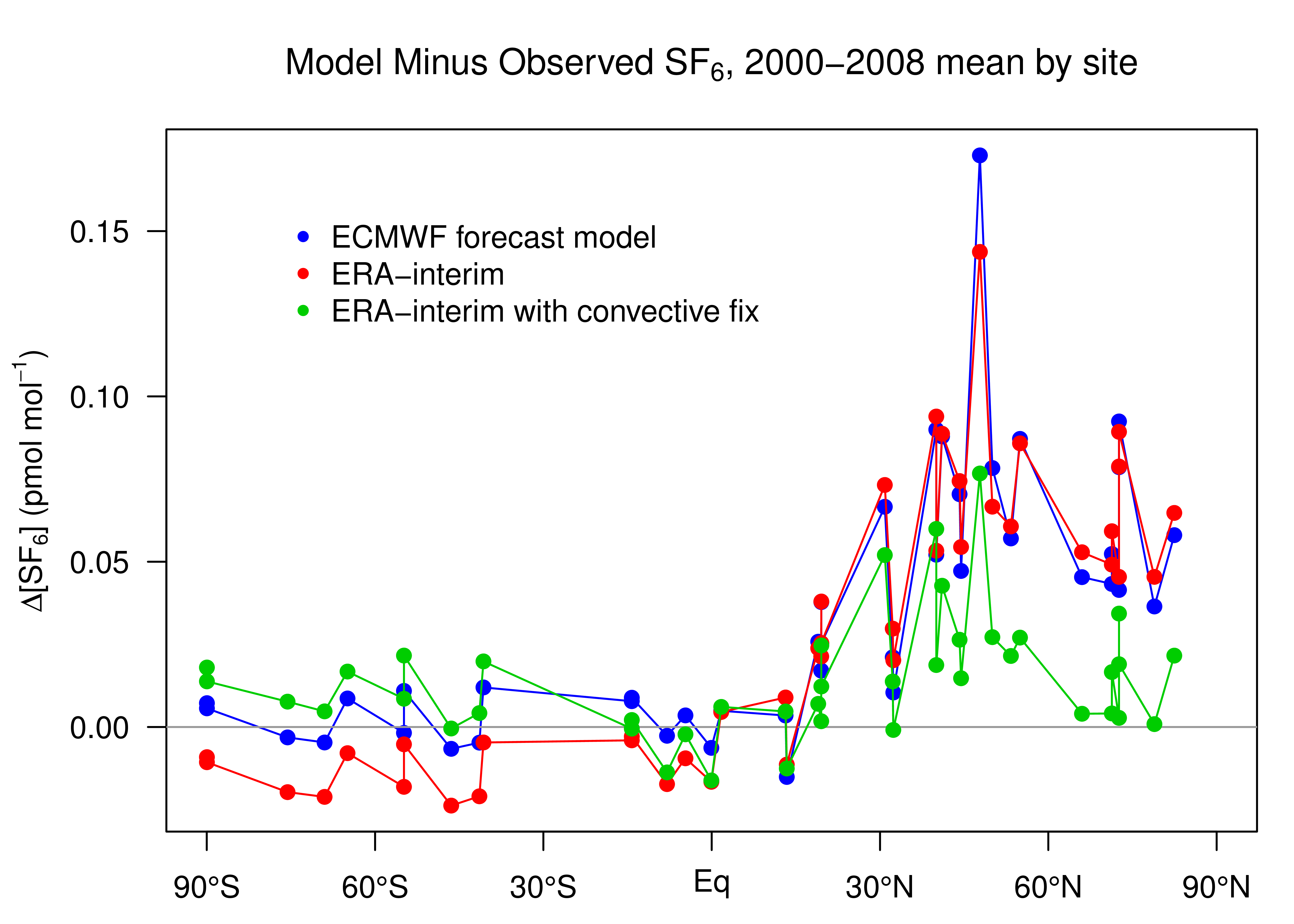
Figure 12: Long-term mean model residuals of SF6 concentrations
as a function of latitude. Residuals are defined as
model-minus-observation, so a positive residual indicates the model
has too much SF6. Three different transport model
simulations are shown. The ECMWF forecast (blue) and ERA-interim
(red) transport simulations do not include the recent "convective
flux fix". The ERA-interim with this convective flux fix is shown
in green. Units are pmol mol−1, or parts per trillion. CT2019B uses
the ERA-interim transport with the convective flux
fix.
In a previous configuration of TM5, the convective entrainment and
detrainment mass fluxes of the parent ECMWF model were re-diagnosed
within TM5 using other meteorological information. The ECMWF model is
used to produce both operational forecasts and the ERA-interim
reanalysis, but the convective fluxes are stored for the ERA-interim
product only. Thus, using ERA-interim meteorology, a direct
comparison is possible. This comparison revealed that the TM5
internal rediagnosis of convective fluxes was faulty. TM5 was
subsequently modified to use parent model ERA-interim convective
fluxes directly. Using the parent model convective fluxes result in a
significantly better SF6 simulations. Simulations with these
parent-model convective fluxes are said to use the "convective flux
fix". Simulations with the convective flux fix show significantly
improved agreement with SF6 observations (see Figure
12).
Since the parent-model convective fluxes are only available for the
ERA-interim product, CT2019B uses only ERA-interim transport with the
convective flux fix. Previous releases of CarbonTracker also used the
ECMWF operational model transport, for which parent-model convective
fluxes are not available. We believe that TM5 simulations without the
parent-model convective fluxes are faulty and should not be included
in our product. When the convective flux fix was instituted in
CT2013B, it resulted in the largest realignment of surface CO2
fluxes in the history of the CarbonTracker program
(Schuh et al., 2019).
This is a prominent example of the sensitive reliance of atmospheric
inversions on accurate atmospheric transport.
7 Observations
The observations of atmospheric CO2 mole fraction made by NOAA ESRL and partner laboratories are at the heart of CarbonTracker. They inform us on changes in the carbon cycle, whether those changes are regular (such as the annual cycle of growth and decay of leaves and other plant matter), or irregular (such as the release of tons of carbon by a wildfire). The results in CarbonTracker depend directly on the quality, location, and frequency of avaiable observations. The level of detail at which we can retrieve information on the carbon cycle increases strongly with the density of the CO2 observing network.7.1 The CarbonTracker observational network
Observations simulated by CT2019B are suppplied by the GLOBALVIEW+ data product version 5.0 (Cooperative Global Atmospheric Data Integration Project, 2019), available at the NOAA ESRL ObsPack web site. This study uses measurements of air samples collected at 460 sites around the world by 55 laboratories:- Commonwealth Scientific and Industrial Research Organization, Oceans & Atmosphere Flagship - GASLAB (CSIRO)
- Instituto de Pesquisas Energeticas e Nucleares (IPEN)
- Environment and Climate Change Canada (ECCC)
- Finnish Meteorological Institute (FMI)
- Laboratoire des Sciences du Climat et de l'Environnement - UMR8212 CEA-CNRS-UVSQ (LSCE)
- University of Heidelberg, Institut für Umweltphysik (UHEI-IUP)
- Umweltbundesamt, Station Schauinsland (UBA-SCHAU)
- Hungarian Meteorological Service (HMS)
- Center for Atmospheric and Oceanic Studies, Tohoku University (TU)
- Meteorological Research Institute (MRI)
- Japan Meteorological Agency (JMA)
- National Institute for Environmental Studies (NIES)
- Comprehensive Observation Network for TRace gases by AirLiner (CONTRAIL)
- University of Groningen (RUG), Centre for Isotope Research (CIO) (RUG)
- Energy Research Centre of the Netherlands (ECN)
- National Institute of Water and Atmospheric Research (NIWA)
- University of Science and Technology (AGH)
- South African Weather Service (SAWS)
- Izana Atmospheric Research Center, Meteorological State Agency of Spain (AEMET)
- Swiss Federal Laboratories for Materials Science and Technology (EMPA)
- World Meteorological Organization/Global Atmosphere Watch (WMO/GAW)
- University of Bern, Physics Institute, Climate and Environmental Physics (KUP)
- University of East Anglia (UEA)
- NOAA Global Monitoring Division (NOAA)
- National Center For Atmospheric Research (NCAR)
- Scripps Institution of Oceanography (SIO)
- Harvard University (HU)
- Lawrence Berkeley National Laboratory and ARM Climate Research Facility (LBNL-ARM)
- HIAPER Pole-to-Pole Observations project (HIPPO)
- University of Wisconsin (UOFWI)
- Savannah River National Laboratory (SRNL)
- Lawrence Berkeley National Laboratory (LBNL)
- National Institute for Space Research (INPE)
- University of Helsinki (UHELS)
- Hohenpeissenberg Meteorological Observatory (HPB)
- Ricerca sul Sistema Energetico (RSE)
- Institut de Ciencia i Tecnologia Ambientals, Universitat Autonoma de Barcelona (ICTA-UAB)
- Lund University - Centre for Environmental and Climate Research (LUND-CEC)
- CarboCount-CH (CARBOCOUNT-CH)
- AVOCET Group @ NASA LaRC (NASA-LARC)
- Penn State University (PSU)
- Oregon State University (OSU)
- NOAA ESRL Halocarbons and Other Atmospheric Trace Species (NOAA-HATS)
- AmeriFlux Network (AMERIFLUX)
- University of Minnesota (UOFMN)
- NOAA Chemical Sciences Division (NOAA-CSD)
- California Institute of Technology, Division of Geological and Planetary Science (CALTECH)
- University of Virginia (UOFVA)
- Indianapolis Flux Experiment (INFLUX)
- Carbon in Arctic Reservoirs Vulnerability Experiment, NASA Earth Ventures (CARVE)
- Utah Atmospheric Trace gas & Air Quality (U-ATAQ)
- NASA Goddard Space Flight Center (NASA-GSFC)
| Source | Online availability | Comment |
| GLOBALVIEW+ v5.0 | ObsPack download | Main source of observations |
| NRT v5.0 | ObsPack download | Measurements in 2019, after end of GLOBALVIEW+ 5.0 |
| NIES shipboard observations | Available from NIES | No permission to redistribute |
| NIES JR-STATION Siberia towers | Download from NIES website or Available upon request to Motoki Sasakawa; ask for access to JR-STATION restricted ObsPack | No permission to redistribute. See Sasakawa et al. (2010), Sasakawa et al. (2013) |
| AirCore | Available upon request to Colm Sweeney; ask for access to AirCore restricted ObsPack | No permission to redistribute |
| INPE (Brazil) aircraft data | Available upon request to Luciana Gatti; ask for access to INPE restricted ObsPack | No permission to redistribute |
Table 2: Sources of CO2 observational data for CT2019B
We also make available an ObsPack containing the simulated values of
all measurement data considered by CT2019B. This
CT2019B
ObsPack contains most, but not all, of the measured
values. Measured values are only distributed directly when we have
permission to do so.
Users are encouraged to review the usage requirements for these data
products, and to contact the measurement laboratories directly for
details about the observations.
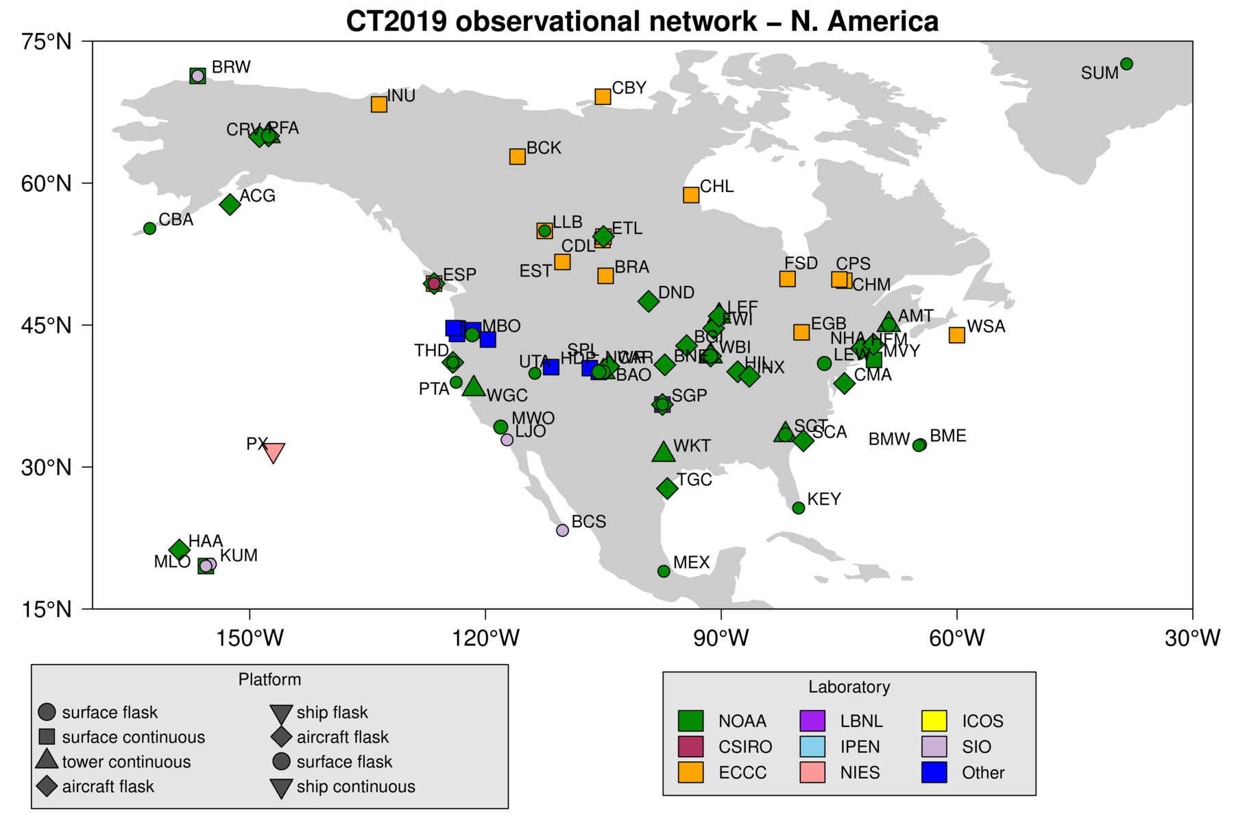
Figure 13: CarbonTracker observational network over North America. See
the CarbonTracker
interactive
network map for more details.
With the advent in 2015 of GLOBALVIEW+, data are now presented to
CarbonTracker with a higher temporal frequency than in past
observational products. At sites with quasi-continuous monitoring,
CT2019B now assimilates hourly average CO2 concentrations. In the
past, a single daily assimilation value was constructed at these
sites, generally a four-hour average during well-mixed background
conditions. At continental sites, this four-hour period was generally
from local noon to 4pm; at many mountain sites background conditions
are met at nighttime when upslope winds are uncommon. With GLOBALVIEW+,
CarbonTracker now assimilates each hourly average during these
background conditions independently. For many sites, all available
hourly averages throughout the day are assimilated. Details vary by
dataset, but can be checked at the interactive data
plotting page.
Note that all of these observations are calibrated against the same
world CO2 standard (WMO-X2007).
Starting with GLOBALVIEW+, we generally use the recommendations of
data providers as to which observations are appropriate for
assimilation. Such observations are identified by a variable in the
ObsPack distribution, obs_flag. Only observations with obs_flag = 1
are identified for assimilation by data providers. We modify the
designation of assimilation data for Environment and Climate Change
Canada quasi-continuous sampling sites. For these data, obs_flag is
set to 1 by the data provider for times when they represent the daily
minimum CO2 concentration. This is generally later in the day
than our standard scheme of local noon-4pm used to represent times of
well-mixed PBLs. For these datasets, we have changed obs_flag to
indicate assimilation only for the local noon - 4pm time period.
These selected observations are further filtered based on the CCG
curve fitting routine of
Thoning et al. (1989). This filter fits a
smooth curve to the selected observations, and measurements more than
3 standard deviations away from this curve are excluded from
assimilation.
At mountain-top sites (e.g. MLO, NWR, and SPL), it is usually
nighttime hours that are selected for assimilation, as these tend to
be the most stable time period. Nighttime hours also avoid periods of
upslope flows that contain local vegetative and/or anthropogenic
influence.
Data from the Sutro tower (STR) and the Boulder (Erie, Colorado) tower
(BAO) are strongly influenced by local urban emissions, which
CarbonTracker is unable to resolve. At these two sites, pollution
events have been identified using co-located measurements of carbon
monoxide. In this study, measurements thought to be affected by
pollution events have been excluded. This technique is under active
refinement.
With CT2019B, we have begun to assimilate CO2 measurements from
NOAA light aircraft profiling time series, from intakes at multiple
levels on NOAA tall towers, and from extensive shipboard and Siberian
tower measurements collected by our partners at NIES. These datasets
can be explored at the interactive data plotting
page.
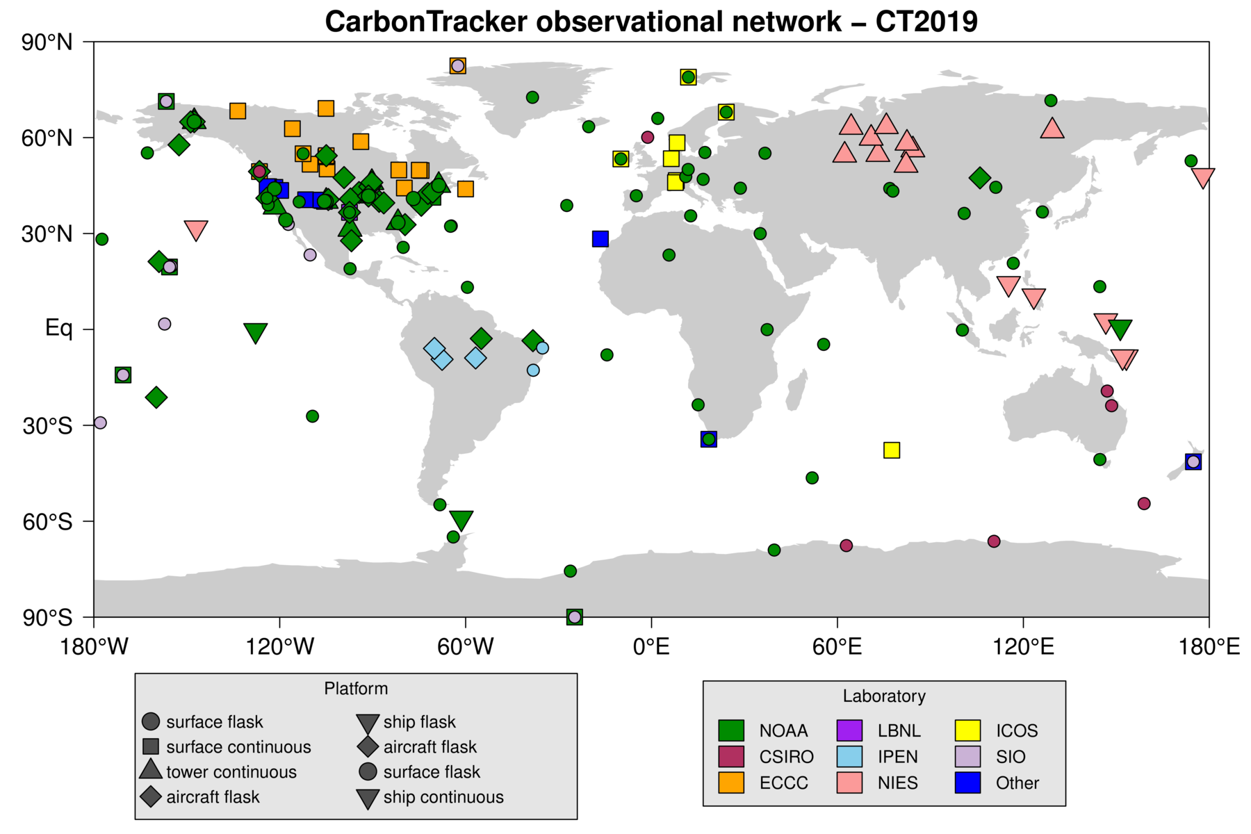
Figure 14: CarbonTracker global observational network. See
the CarbonTracker
interactive
network map for more details.
We apply a further selection criterion during the assimilation to
exclude non-marine boundary layer (MBL) observations that are very
poorly forecasted in our framework. We use the so-called model-data
mismatch in this process, which is the random error ascribed to each
observation to account for measurement errors as well as modeling errors
of that observation. We interpret an observed-minus-forecasted
mole fraction that exceeds 3 times the prescribed model-data mismatch as
an indicator that our modeling framework fails. This can happen for
instance when an air sample is representative of local exchange not
captured well by our 1° × 1° fluxes, when local meteorological
conditions are not captured by our offline transport fields, but also
when large-scale CO2 exchange is suddenly changed (e.g. fires, pests,
droughts) to an extent that can not be accommodated by our flux modules.
This last situation would imply an important change in the carbon cycle
and has to be recognized by the researchers when analyzing the results.
In accordance with the 3-sigma rejection criterion, about 0.2%
of the observations are discarded through this mechanism in our
assimilations.
7.2 Adaptive model-data mismatch
The statistical optimization method we use to constrain surface CO2 fluxes requires that each assimilation constraint is assigned a "model-data mismatch" (MDM) error value. This is meant to express the statistics of simulated-minus-observed CO2 observations we could expect if CarbonTracker were using perfect surface fluxes. Such deviations arise from many sources, including random noise in the measurement system, in situ variability that we do not expect to resolve in our model, and faults with the atmospheric transport model. Generally, transport and inverse model faults are the dominant terms in MDM values. The MDM is one of two major "tuning knobs" used to adjust the performance of our ensemble Kalman filter. The other is also an error quantity, meant to represent the expected error on our first-guess fluxes. Discussion of this prior covariance error can be found in section 8.2. Prior to CT2015, CarbonTracker used a single MDM value for each assimilation dataset. The NOAA continuous observations at the 396m level of the WLEF tower in northern Wisconsin, for example, were assigned a MDM of 3.0 ppm, meaning that the residuals between model-forecasted measurements and the actual observed concentrations are expected to be unbiased (i.e., have a mean of zero) and have a standard deviation of 3 ppm. In practice, however, we have found that it is far easier to simulate wintertime observations than those during summer. This is mainly due to higher ambient variability of CO2 in the summer. Starting with CT2016, we began to use an empirical scheme to assign MDM values, exploiting statistics of model performance from indenpendently-configured preliminary inversions. The posterior residuals for each dataset are classified into relevant bins, and then statistics of model performance are analyzed within each of those bins. For every dataset, these bins include equally-spaced intervals of one-tenth of a year. For analyzers collecting data throughout the day, we also classify the measurements into 4-hour intervals of local time. For aircraft datasets, we further classify measurements into vertical levels of 1000m thickness (0-1000 m ASL, 1000-2000 m ASL, etc.). For each of these bins, bias and random error are combined to form total deviation from observed values as a root-mean square error (RMSE). The assigned MDM is set to a constant fraction of this total RMSE. This scaling is meant to force the assimilation scheme to extract as much information as possible from available observations. We use two different scaling factors to convert RMSE to MDM, depending on whether the preliminary inversions actually assimilated the measurements in the relevant bin, or merely simulated those measurements. For measurements assimilated by the preliminary inversions, the MDM is 0.95 * RMSE; for measurements not assimilated in the preliminary inversions, the MDM is 0.85 * RMSE. The adaptive MDM scheme performs well in terms of average χ2, which in an optimally-tuned system should be close to 1.0 for each dataset (see Table 3). Notably, the seasonal variations of MDM successfully compensate for the higher ambient variability of CO2 at continental sites during the growing season. It is, however, an iterative process, requiring that we conduct a previous inversion. For various reasons, this previous inversion performed before CT2019B differs in significant aspects from the actual CT2019B inversions. These differences have led to MDM values which are slightly too large and thus average χ2 values which are generally smaller than the target of 1.0 (in some cases, as low as 0.2 or 0.3). The next iteration of CarbonTracker will be able to use the more recent CT2019B inversions to refine the adaptive MDM scheme. Duplicate observations are identified as those within 50 minutes temporally, 10m vertically, and 0.05 degrees of latitude and longitude laterally (nominally, about 5km). The MDM for such observations is inflated by √n, where n is the number of duplicates.7.3 Statistical performance of CT2019B
Starting with CT2019B, we reserved about 5% of available assimilation data for a cross-validation exercise. To the extent possible, withheld measurements were chosen to be independent from other observations. For surface flask observations, which are generally collected on a weekly time basis, all samoples are considered independent from one another, so withheld data were selected randomly. Aircraft flasks collected during a profile are considered co-dependent, so entire profiles were randomly selected for withholding. Finally, for in situ analyzers with quasi-continuous sampling (towers, observatories), 24-hour periods were randomly chosen and that entire day's worth of data were withheld. Shipboard quasi-continuous datasets, which account for more than a quarter of assimilation data for CT2019B were inadvertently excluded from this cross-validation exercise. As a result, about 3% (115,756 measurements out of about 4.2 million) were withheld. Each residual from the withheld measurements was normalized by its prescribed model-data mismatch (MDM) error, to form a set of χ values. The mean χ2, which for a perfect set of independent, normally-distributed variates should approach 1.0, was found to be 0.92. Table 3 summarizes the datasets assimilated in CarbonTracker, and the performace of the assimilation scheme for each dataset. These diagnostics are useful for evaluating how well CarbonTracker does in simulating observed CO2.| Dataset | Lab. | Location | Latitude | Longitude | Elev. | Used | Rej. | Unsampled | R | χ2 | Bias | SE |
| (m) | (ppm) | (ppm) | (ppm) | |||||||||
| co2_abp_surface-flask_1_representative | NOAA | Arembepe, Bahia, Brazil | 12.77°S | 38.17°W | 1 | 88 | 0 | 0 | 1.0 - 2.9 | 0.47 | -1.03 | 0.96 |
| co2_abp_surface-flask_26_marine | IPEN | Arembepe, Bahia, Brazil | 12.77°S | 38.17°W | 1 | 88 | 3 | 0 | 0.5 - 4.6 | 0.66 | -2.88 | 12.89 |
| co2_acg_aircraft-pfp_1_allvalid_0-1000masl | NOAA | Alaska Coast Guard, United States | 57.74°N | 152.50°W | 440 | 413 | 22 | 0 | 0.2 - 4.9 | 1.10 | -0.41 | 2.62 |
| co2_acg_aircraft-pfp_1_allvalid_1000-2000masl | NOAA | Alaska Coast Guard, United States | 57.74°N | 152.50°W | 1490 | 229 | 7 | 0 | 0.5 - 4.9 | 1.10 | -0.03 | 1.79 |
| co2_acg_aircraft-pfp_1_allvalid_2000-3000masl | NOAA | Alaska Coast Guard, United States | 57.74°N | 152.50°W | 2533 | 147 | 1 | 0 | 0.5 - 3.2 | 1.05 | 0.08 | 1.36 |
| co2_acg_aircraft-pfp_1_allvalid_3000-4000masl | NOAA | Alaska Coast Guard, United States | 57.74°N | 152.50°W | 3530 | 136 | 1 | 0 | 0.5 - 4.9 | 1.00 | 0.31 | 1.33 |
| co2_acg_aircraft-pfp_1_allvalid_4000-5000masl | NOAA | Alaska Coast Guard, United States | 57.74°N | 152.50°W | 4424 | 124 | 1 | 0 | 0.5 - 4.9 | 0.81 | -0.05 | 1.25 |
| co2_acg_aircraft-pfp_1_allvalid_5000-6000masl | NOAA | Alaska Coast Guard, United States | 57.74°N | 152.50°W | 5494 | 133 | 2 | 0 | 0.5 - 4.9 | 0.70 | 0.09 | 1.29 |
| co2_acg_aircraft-pfp_1_allvalid_6000-7000masl | NOAA | Alaska Coast Guard, United States | 57.74°N | 152.50°W | 6443 | 131 | 3 | 0 | 0.5 - 4.9 | 0.89 | 0.22 | 1.33 |
| co2_acg_aircraft-pfp_1_allvalid_7000-8000masl | NOAA | Alaska Coast Guard, United States | 57.74°N | 152.50°W | 7495 | 156 | 1 | 1 | 0.3 - 3.2 | 0.84 | 0.03 | 1.36 |
| co2_acg_aircraft-pfp_1_allvalid_8000-9000masl | NOAA | Alaska Coast Guard, United States | 57.74°N | 152.50°W | 8342 | 24 | 0 | 0 | 0.7 - 3.0 | 0.74 | 0.45 | 0.93 |
| co2_ah2_shipboard-insitu_20_allvalid | NIES | Alligator Hope (M/S Alligator Hope of Mitsui O.S.K. Lines, Ltd.) | variable | Surface | 29521 | 2764 | 14 | 0.2 - 100.6 | 0.97 | -0.34 | 2.91 | |
| co2_alf_aircraft-pfp_26_representative_0-1000masl | IPEN | Alta Floresta, Brazil | 8.92°S | 56.79°W | 677 | 159 | 0 | 0 | 1.3 - 6.9 | 0.95 | -1.20 | 4.22 |
| co2_alf_aircraft-pfp_26_representative_1000-2000masl | IPEN | Alta Floresta, Brazil | 8.92°S | 56.79°W | 1526 | 171 | 2 | 0 | 1.3 - 6.1 | 1.01 | -0.28 | 2.81 |
| co2_alf_aircraft-pfp_26_representative_2000-3000masl | IPEN | Alta Floresta, Brazil | 8.92°S | 56.79°W | 2379 | 105 | 1 | 0 | 0.8 - 4.4 | 0.95 | -0.37 | 1.68 |
| co2_alf_aircraft-pfp_26_representative_3000-4000masl | IPEN | Alta Floresta, Brazil | 8.92°S | 56.79°W | 3504 | 179 | 3 | 0 | 0.6 - 3.1 | 1.03 | -0.06 | 1.63 |
| co2_alf_aircraft-pfp_26_representative_4000-5000masl | IPEN | Alta Floresta, Brazil | 8.92°S | 56.79°W | 4420 | 54 | 1 | 0 | 0.7 - 2.4 | 1.16 | 0.35 | 1.42 |
| co2_alt_surface-flask_1_representative | NOAA | Alert, Nunavut, Canada | 82.45°N | 62.51°W | 190 | 956 | 30 | 0 | 0.2 - 5.1 | 0.67 | 0.02 | 0.87 |
| co2_alt_surface-flask_2_representative | CSIRO | Alert, Nunavut, Canada | 82.45°N | 62.51°W | 190 | 608 | 38 | 0 | 0.2 - 1.9 | 1.08 | 0.08 | 0.97 |
| co2_alt_surface-flask_4_representative | SIO | Alert, Nunavut, Canada | 82.45°N | 62.51°W | 190 | 397 | 25 | 0 | 0.4 - 4.4 | 0.76 | 0.17 | 0.84 |
| co2_alt_surface-flask_426_representative | SIO_CO2 | Alert, Nunavut, Canada | 82.45°N | 62.51°W | 190 | 584 | 11 | 0 | 0.5 - 5.9 | 0.65 | 0.00 | 0.96 |
| co2_alt_surface-insitu_6_allvalid | EC | Alert, Nunavut, Canada | 82.45°N | 62.51°W | 190 | 21929 | 1384 | 0 | 0.5 - 4.1 | 1.01 | -0.00 | 0.83 |
| co2_ams_surface-insitu_11_representative | LSCE | Amsterdam Island, France | 37.80°S | 77.54°E | 55 | 126717 | 2302 | 0 | 0.3 - 1.0 | 0.78 | -0.10 | 0.57 |
| co2_amt_surface-pfp_1_allvalid-107magl | NOAA | Argyle, Maine, United States | 45.03°N | 68.68°W | 53 | 1401 | 7 | 0 | 1.5 - 13.2 | 0.41 | 0.34 | 3.42 |
| co2_amt_tower-insitu_1_allvalid-107magl | NOAA | Argyle, Maine, United States | 45.03°N | 68.68°W | 53 | 18481 | 420 | 0 | 1.5 - 8.5 | 0.74 | 0.27 | 3.54 |
| co2_amt_tower-insitu_1_allvalid-12magl | NOAA | Argyle, Maine, United States | 45.03°N | 68.68°W | 53 | 18047 | 455 | 0 | 1.5 - 6.6 | 0.83 | 0.47 | 4.02 |
| co2_amt_tower-insitu_1_allvalid-30magl | NOAA | Argyle, Maine, United States | 45.03°N | 68.68°W | 53 | 12289 | 344 | 0 | 1.5 - 6.7 | 0.87 | 0.81 | 3.85 |
| co2_ara_surface-flask_2_representative | CSIRO | Arcturus, Queensland, Australia | 23.86°S | 148.47°E | 175 | 11 | 0 | 0 | 1.7 - 10.0 | 0.18 | 0.08 | 2.41 |
| co2_asc_surface-flask_1_representative | NOAA | Ascension Island, United Kingdom | 7.97°S | 14.40°W | 85 | 1524 | 0 | 0 | 0.5 - 1.0 | 1.49 | 0.10 | 0.78 |
| co2_ask_surface-flask_1_representative | NOAA | Assekrem, Algeria | 23.26°N | 5.63°E | 2710 | 814 | 10 | 0 | 0.2 - 1.0 | 0.99 | -0.12 | 0.62 |
| co2_azr_surface-flask_1_representative | NOAA | Terceira Island, Azores, Portugal | 38.77°N | 27.38°W | 19 | 465 | 12 | 0 | 0.4 - 2.5 | 0.99 | 0.18 | 1.37 |
| co2_azv_tower-insitu_20_allvalid-29magl | NIES | Azovo, Russia | 54.70°N | 73.03°E | 110 | 10113 | 220 | 0 | 1.9 - 6.0 | 0.93 | -0.77 | 3.70 |
| co2_azv_tower-insitu_20_allvalid-50magl | NIES | Azovo, Russia | 54.70°N | 73.03°E | 110 | 9758 | 211 | 0 | 1.9 - 6.0 | 0.93 | -0.65 | 3.69 |
| co2_bal_surface-flask_1_representative | NOAA | Baltic Sea, Poland | 55.35°N | 17.22°E | 3 | 907 | 13 | 0 | 0.4 - 11.3 | 0.73 | -1.97 | 5.57 |
| co2_bao_surface-pfp_1_allvalid-300magl | NOAA | Boulder Atmospheric Observatory, Colorado, United States | 40.05°N | 105.00°W | 1584 | 2136 | 2 | 0 | 2.5 - 29.7 | 0.39 | -1.77 | 2.98 |
| co2_bao_tower-insitu_1_allvalid-100magl | NOAA | Boulder Atmospheric Observatory, Colorado, United States | 40.05°N | 105.00°W | 1584 | 9931 | 309 | 0 | 2.3 - 9.5 | 0.82 | -3.44 | 6.60 |
| co2_bao_tower-insitu_1_allvalid-22magl | NOAA | Boulder Atmospheric Observatory, Colorado, United States | 40.05°N | 105.00°W | 1584 | 10045 | 292 | 0 | 2.4 - 12.6 | 0.80 | -4.02 | 8.23 |
| co2_bao_tower-insitu_1_allvalid-300magl | NOAA | Boulder Atmospheric Observatory, Colorado, United States | 40.05°N | 105.00°W | 1584 | 65994 | 1103 | 0 | 2.2 - 78.3 | 0.77 | 0.29 | 5.65 |
| co2_bck_surface-insitu_6_allvalid | EC | Behchoko, Northwest Territories, Canada | 62.80°N | 115.92°W | 160 | 8692 | 385 | 0 | 1.7 - 9.2 | 0.78 | 0.05 | 2.37 |
| co2_bcs_surface-flask_426_representative | SIO_CO2 | Baja California Sur, Mexico | 23.30°N | 110.20°W | 4 | 112 | 2 | 0 | 0.6 - 6.5 | 0.53 | 0.66 | 1.97 |
| co2_bgi_aircraft-pfp_1_allvalid_0-1000masl | NOAA | Bradgate, Iowa, United States | 42.82°N | 94.41°W | 612 | 8 | 0 | 0 | 2.2 - 8.8 | 0.60 | -2.34 | 5.09 |
| co2_bgi_aircraft-pfp_1_allvalid_1000-2000masl | NOAA | Bradgate, Iowa, United States | 42.82°N | 94.41°W | 1565 | 53 | 4 | 0 | 0.5 - 6.9 | 0.79 | -1.11 | 2.62 |
| co2_bgi_aircraft-pfp_1_allvalid_2000-3000masl | NOAA | Bradgate, Iowa, United States | 42.82°N | 94.41°W | 2548 | 16 | 0 | 0 | 0.5 - 1.9 | 1.06 | -0.16 | 1.11 |
| co2_bgi_aircraft-pfp_1_allvalid_3000-4000masl | NOAA | Bradgate, Iowa, United States | 42.82°N | 94.41°W | 3524 | 50 | 2 | 0 | 0.2 - 3.0 | 1.27 | 0.24 | 1.23 |
| co2_bgi_aircraft-pfp_1_allvalid_4000-5000masl | NOAA | Bradgate, Iowa, United States | 42.82°N | 94.41°W | 4569 | 26 | 0 | 0 | 0.2 - 1.4 | 1.37 | 0.28 | 0.69 |
| co2_bgi_aircraft-pfp_1_allvalid_5000-6000masl | NOAA | Bradgate, Iowa, United States | 42.82°N | 94.41°W | 5506 | 36 | 6 | 0 | 0.0 - 1.8 | 1.28 | 0.22 | 0.89 |
| co2_bgi_aircraft-pfp_1_allvalid_6000-7000masl | NOAA | Bradgate, Iowa, United States | 42.82°N | 94.41°W | 6474 | 38 | 0 | 0 | 0.5 - 1.9 | 1.15 | 0.14 | 1.19 |
| co2_bgi_aircraft-pfp_1_allvalid_7000-8000masl | NOAA | Bradgate, Iowa, United States | 42.82°N | 94.41°W | 7469 | 39 | 0 | 0 | 0.2 - 1.3 | 1.19 | 0.09 | 0.68 |
| co2_bgi_aircraft-pfp_1_allvalid_8000-9000masl | NOAA | Bradgate, Iowa, United States | 42.82°N | 94.41°W | 8050 | 3 | 0 | 0 | 0.8 - 0.8 | 0.85 | -0.08 | 1.19 |
| co2_bhd_surface-flask_1_representative | NOAA | Baring Head Station, New Zealand | 41.41°S | 174.87°E | 85 | 222 | 3 | 0 | 0.2 - 2.8 | 0.78 | 0.08 | 1.28 |
| co2_bhd_surface-flask_426_representative | SIO_CO2 | Baring Head Station, New Zealand | 41.41°S | 174.87°E | 85 | 130 | 3 | 0 | 0.3 - 5.7 | 1.01 | 1.08 | 1.26 |
| co2_bhd_surface-insitu_15_baseline | NIWA | Baring Head Station, New Zealand | 41.41°S | 174.87°E | 85 | 595 | 20 | 0 | 0.4 - 2.7 | 1.02 | 0.65 | 1.24 |
| co2_bir_surface-insitu_56_allvalid | NILU | Birkenes Observatory, Norway | 58.39°N | 8.25°E | 219 | 1291 | 29 | 0 | 1.6 - 5.9 | 0.76 | 0.75 | 3.08 |
| co2_bkt_surface-flask_1_representative | NOAA | Bukit Kototabang, Indonesia | 0.20°S | 100.32°E | 845 | 441 | 1 | 0 | 4.6 - 6.6 | 0.98 | 4.36 | 3.73 |
| co2_bme_surface-flask_1_representative | NOAA | St. Davids Head, Bermuda, United Kingdom | 32.37°N | 64.65°W | 12 | 213 | 7 | 0 | 0.7 - 2.9 | 0.98 | 0.53 | 1.58 |
| co2_bmw_surface-flask_1_representative | NOAA | Tudor Hill, Bermuda, United Kingdom | 32.26°N | 64.88°W | 30 | 589 | 24 | 0 | 0.4 - 2.1 | 1.06 | 0.64 | 1.30 |
| co2_bne_aircraft-pfp_1_allvalid_0-1000masl | NOAA | Beaver Crossing, Nebraska, United States | 40.80°N | 97.18°W | 634 | 73 | 1 | 0 | 2.6 - 10.8 | 0.75 | -0.21 | 4.54 |
| co2_bne_aircraft-pfp_1_allvalid_1000-2000masl | NOAA | Beaver Crossing, Nebraska, United States | 40.80°N | 97.18°W | 1393 | 183 | 4 | 0 | 0.6 - 8.7 | 0.99 | -0.31 | 2.62 |
| co2_bne_aircraft-pfp_1_allvalid_2000-3000masl | NOAA | Beaver Crossing, Nebraska, United States | 40.80°N | 97.18°W | 2296 | 110 | 3 | 0 | 0.3 - 9.8 | 0.92 | -0.54 | 2.02 |
| co2_bne_aircraft-pfp_1_allvalid_3000-4000masl | NOAA | Beaver Crossing, Nebraska, United States | 40.80°N | 97.18°W | 3393 | 147 | 3 | 0 | 0.2 - 10.0 | 1.05 | -0.23 | 1.71 |
| co2_bne_aircraft-pfp_1_allvalid_4000-5000masl | NOAA | Beaver Crossing, Nebraska, United States | 40.80°N | 97.18°W | 4280 | 81 | 2 | 0 | 0.4 - 12.8 | 1.03 | -0.33 | 2.36 |
| co2_bne_aircraft-pfp_1_allvalid_5000-6000masl | NOAA | Beaver Crossing, Nebraska, United States | 40.80°N | 97.18°W | 5392 | 118 | 3 | 0 | 0.3 - 14.8 | 0.95 | -0.16 | 2.20 |
| co2_bne_aircraft-pfp_1_allvalid_6000-7000masl | NOAA | Beaver Crossing, Nebraska, United States | 40.80°N | 97.18°W | 6362 | 113 | 2 | 0 | 0.2 - 15.2 | 1.24 | -0.12 | 2.26 |
| co2_bne_aircraft-pfp_1_allvalid_7000-8000masl | NOAA | Beaver Crossing, Nebraska, United States | 40.80°N | 97.18°W | 7657 | 86 | 2 | 0 | 0.1 - 23.3 | 1.15 | 0.28 | 0.74 |
| co2_bne_aircraft-pfp_1_allvalid_8000-9000masl | NOAA | Beaver Crossing, Nebraska, United States | 40.80°N | 97.18°W | 8072 | 24 | 1 | 0 | 0.4 - 1.2 | 0.70 | -0.21 | 0.80 |
| co2_bra_surface-insitu_6_allvalid | EC | Bratt's Lake Saskatchewan, Canada | 50.20°N | 104.71°W | 595 | 8611 | 191 | 0 | 2.3 - 8.6 | 0.80 | 0.06 | 2.74 |
| co2_brw_surface-flask_1_representative | NOAA | Barrow Atmospheric Baseline Observatory, United States | 71.32°N | 156.61°W | 11 | 989 | 10 | 3 | 0.8 - 10.9 | 0.46 | -0.23 | 1.77 |
| co2_brw_surface-flask_426_representative | SIO_CO2 | Barrow Atmospheric Baseline Observatory, United States | 71.32°N | 156.61°W | 11 | 655 | 7 | 0 | 0.7 - 16.2 | 0.73 | -0.01 | 1.75 |
| co2_brw_surface-insitu_1_allvalid | NOAA | Barrow Atmospheric Baseline Observatory, United States | 71.32°N | 156.61°W | 11 | 31993 | 951 | 0 | 1.4 - 7.4 | 0.65 | -0.08 | 1.41 |
| co2_brz_aircraft-insitu_20_allvalid_0-1000masl | NIES | Berezorechka, Russia | 56.15°N | 84.33°E | 636 | 32953 | 99 | 0 | 1.2 - 156.0 | 0.25 | -0.63 | 3.32 |
| co2_brz_aircraft-insitu_20_allvalid_1000-2000masl | NIES | Berezorechka, Russia | 56.15°N | 84.33°E | 1501 | 44112 | 113 | 0 | 1.2 - 88.5 | 0.17 | -0.56 | 2.73 |
| co2_brz_aircraft-insitu_20_allvalid_2000-3000masl | NIES | Berezorechka, Russia | 56.15°N | 84.33°E | 2408 | 20179 | 52 | 0 | 1.2 - 114.8 | 0.14 | -0.57 | 2.43 |
| co2_brz_aircraft-insitu_20_allvalid_3000-4000masl | NIES | Berezorechka, Russia | 56.15°N | 84.33°E | 3085 | 2750 | 1 | 0 | 1.2 - 62.2 | 0.14 | -0.52 | 2.61 |
| co2_brz_tower-insitu_20_allvalid-20magl | NIES | Berezorechka, Russia | 56.15°N | 84.33°E | 168 | 13338 | 312 | 0 | 2.3 - 24.6 | 0.80 | -0.22 | 3.79 |
| co2_brz_tower-insitu_20_allvalid-40magl | NIES | Berezorechka, Russia | 56.15°N | 84.33°E | 168 | 13325 | 280 | 0 | 2.2 - 23.8 | 0.82 | -0.43 | 3.84 |
| co2_brz_tower-insitu_20_allvalid-5magl | NIES | Berezorechka, Russia | 56.15°N | 84.33°E | 168 | 13493 | 290 | 0 | 2.3 - 25.0 | 0.81 | -0.24 | 3.84 |
| co2_brz_tower-insitu_20_allvalid-80magl | NIES | Berezorechka, Russia | 56.15°N | 84.33°E | 168 | 8392 | 204 | 0 | 1.9 - 24.3 | 0.89 | -0.69 | 3.94 |
| co2_bsc_surface-flask_1_representative | NOAA | Black Sea, Constanta, Romania | 44.18°N | 28.66°E | 0 | 405 | 4 | 0 | 1.8 - 20.7 | 0.99 | -5.92 | 8.11 |
| co2_car_aircraft-pfp_1_allvalid_1000-2000masl | NOAA | Briggsdale, Colorado, United States | 40.63°N | 104.33°W | 1788 | 34 | 0 | 0 | 1.3 - 5.1 | 1.20 | -0.95 | 2.49 |
| co2_car_aircraft-pfp_1_allvalid_2000-3000masl | NOAA | Briggsdale, Colorado, United States | 40.63°N | 104.33°W | 2441 | 917 | 25 | 0 | 0.7 - 7.3 | 0.78 | 0.32 | 2.07 |
| co2_car_aircraft-pfp_1_allvalid_3000-4000masl | NOAA | Briggsdale, Colorado, United States | 40.63°N | 104.33°W | 3460 | 1090 | 42 | 0 | 0.2 - 3.9 | 1.12 | 0.20 | 1.01 |
| co2_car_aircraft-pfp_1_allvalid_4000-5000masl | NOAA | Briggsdale, Colorado, United States | 40.63°N | 104.33°W | 4500 | 1008 | 27 | 0 | 0.2 - 1.9 | 1.13 | 0.25 | 0.86 |
| co2_car_aircraft-pfp_1_allvalid_5000-6000masl | NOAA | Briggsdale, Colorado, United States | 40.63°N | 104.33°W | 5484 | 785 | 16 | 0 | 0.2 - 1.8 | 1.21 | 0.15 | 0.85 |
| co2_car_aircraft-pfp_1_allvalid_6000-7000masl | NOAA | Briggsdale, Colorado, United States | 40.63°N | 104.33°W | 6446 | 779 | 33 | 0 | 0.1 - 1.5 | 1.26 | 0.31 | 0.78 |
| co2_car_aircraft-pfp_1_allvalid_7000-8000masl | NOAA | Briggsdale, Colorado, United States | 40.63°N | 104.33°W | 7477 | 793 | 17 | 0 | 0.3 - 1.4 | 1.22 | 0.30 | 0.80 |
| co2_car_aircraft-pfp_1_allvalid_8000-9000masl | NOAA | Briggsdale, Colorado, United States | 40.63°N | 104.33°W | 8217 | 170 | 2 | 0 | 0.2 - 1.7 | 1.39 | 0.22 | 0.71 |
| co2_car_aircraft-pfp_1_allvalid_9000-10000masl | NOAA | Briggsdale, Colorado, United States | 40.63°N | 104.33°W | 9140 | 2 | 0 | 0 | 0.7 - 0.7 | 1.09 | -0.29 | 0.93 |
| co2_car_aircraft-pfp_1_allvalid_11000-12000masl | NOAA | Briggsdale, Colorado, United States | 40.63°N | 104.33°W | 11869 | 4 | 0 | 0 | 0.5 - 0.8 | 0.45 | -0.28 | 0.45 |
| co2_cba_surface-flask_1_representative | NOAA | Cold Bay, Alaska, United States | 55.21°N | 162.72°W | 21 | 1243 | 26 | 0 | 0.8 - 4.6 | 0.97 | -0.95 | 1.72 |
| co2_cba_surface-flask_4_representative | SIO | Cold Bay, Alaska, United States | 55.21°N | 162.72°W | 21 | 347 | 24 | 0 | 0.5 - 6.6 | 0.93 | -0.59 | 2.11 |
| co2_cby_surface-insitu_6_allvalid | EC | Cambridge Bay, Nunavut Territory, Canada | 69.13°N | 105.06°W | 35 | 6851 | 229 | 0 | 1.1 - 4.3 | 0.61 | 0.00 | 1.30 |
| co2_cdl_surface-insitu_6_allvalid | EC | Candle Lake, Saskatchewan, Canada | 53.99°N | 105.12°W | 600 | 8650 | 161 | 0 | 2.0 - 8.1 | 0.68 | 0.34 | 2.61 |
| co2_cfa_surface-flask_2_representative | CSIRO | Cape Ferguson, Queensland, Australia | 19.28°S | 147.06°E | 2 | 318 | 3 | 0 | 0.3 - 2.4 | 0.74 | -0.44 | 1.04 |
| co2_cgo_surface-flask_1_representative | NOAA | Cape Grim, Tasmania, Australia | 40.68°S | 144.69°E | 94 | 628 | 0 | 0 | 0.3 - 4.3 | 0.63 | -0.07 | 0.71 |
| co2_cgo_surface-flask_2_representative | CSIRO | Cape Grim, Tasmania, Australia | 40.68°S | 144.69°E | 94 | 839 | 4 | 0 | 0.2 - 3.3 | 0.41 | -0.19 | 0.64 |
| co2_cgo_surface-flask_4_representative | SIO | Cape Grim, Tasmania, Australia | 40.68°S | 144.69°E | 94 | 372 | 4 | 0 | 0.3 - 3.5 | 0.61 | 0.22 | 0.88 |
| co2_chl_surface-insitu_6_allvalid | EC | Churchill, Manitoba, Canada | 58.74°N | 93.82°W | 29 | 5988 | 144 | 0 | 1.7 - 6.2 | 0.57 | -0.17 | 1.85 |
| co2_chm_surface-insitu_6_allvalid | EC | Chibougamau, Quebec, Canada | 49.69°N | 74.34°W | 393 | 3469 | 116 | 0 | 2.3 - 5.5 | 0.95 | 0.01 | 2.43 |
| co2_chr_surface-flask_1_representative | NOAA | Christmas Island, Republic of Kiribati | 1.70°N | 157.15°W | 0 | 564 | 0 | 0 | 0.4 - 1.7 | 0.79 | -0.20 | 0.60 |
| co2_chr_surface-flask_426_representative | SIO_CO2 | Christmas Island, Republic of Kiribati | 1.70°N | 157.15°W | 0 | 261 | 5 | 0 | 0.4 - 1.5 | 0.93 | -0.41 | 0.86 |
| co2_cib_surface-flask_1_representative | NOAA | Centro de Investigacion de la Baja Atmosfera (CIBA), Spain | 41.81°N | 4.93°W | 845 | 390 | 4 | 0 | 2.0 - 6.2 | 0.85 | 0.43 | 3.34 |
| co2_cma_aircraft-pfp_1_allvalid_0-1000masl | NOAA | Offshore Cape May, New Jersey, United States | 38.83°N | 74.32°W | 634 | 478 | 9 | 0 | 1.7 - 7.4 | 0.90 | -0.41 | 3.15 |
| co2_cma_aircraft-pfp_1_allvalid_1000-2000masl | NOAA | Offshore Cape May, New Jersey, United States | 38.83°N | 74.32°W | 1537 | 285 | 11 | 0 | 0.6 - 6.0 | 0.83 | -0.47 | 2.30 |
| co2_cma_aircraft-pfp_1_allvalid_2000-3000masl | NOAA | Offshore Cape May, New Jersey, United States | 38.83°N | 74.32°W | 2299 | 358 | 7 | 0 | 0.6 - 4.3 | 0.86 | -0.35 | 2.00 |
| co2_cma_aircraft-pfp_1_allvalid_3000-4000masl | NOAA | Offshore Cape May, New Jersey, United States | 38.83°N | 74.32°W | 3443 | 333 | 8 | 0 | 0.4 - 2.5 | 1.24 | 0.22 | 1.25 |
| co2_cma_aircraft-pfp_1_allvalid_4000-5000masl | NOAA | Offshore Cape May, New Jersey, United States | 38.83°N | 74.32°W | 4196 | 166 | 13 | 0 | 0.1 - 3.0 | 1.13 | 0.17 | 1.27 |
| co2_cma_aircraft-pfp_1_allvalid_5000-6000masl | NOAA | Offshore Cape May, New Jersey, United States | 38.83°N | 74.32°W | 5343 | 320 | 10 | 0 | 0.3 - 2.6 | 1.17 | 0.18 | 1.04 |
| co2_cma_aircraft-pfp_1_allvalid_6000-7000masl | NOAA | Offshore Cape May, New Jersey, United States | 38.83°N | 74.32°W | 6266 | 262 | 7 | 0 | 0.4 - 1.6 | 1.15 | 0.09 | 1.00 |
| co2_cma_aircraft-pfp_1_allvalid_7000-8000masl | NOAA | Offshore Cape May, New Jersey, United States | 38.83°N | 74.32°W | 7724 | 239 | 6 | 0 | 0.3 - 1.8 | 1.20 | 0.35 | 0.92 |
| co2_cma_aircraft-pfp_1_allvalid_8000-9000masl | NOAA | Offshore Cape May, New Jersey, United States | 38.83°N | 74.32°W | 8043 | 24 | 1 | 0 | 0.6 - 1.4 | 1.06 | 0.52 | 1.03 |
| co2_con_aircraft-flask_20_allvalid_0-1000masl | NIES | CONTRAIL (Comprehensive Observation Network for TRace gases by AIrLiner) | variable | 824 | 2 | 0 | 0 | 0.7 - 0.7 | 0.01 | 0.00 | 0.03 | |
| co2_con_aircraft-flask_20_allvalid_1000-2000masl | NIES | CONTRAIL (Comprehensive Observation Network for TRace gases by AIrLiner) | variable | 1385 | 6 | 0 | 0 | 0.3 - 0.6 | 0.82 | 0.21 | 0.27 | |
| co2_con_aircraft-flask_20_allvalid_2000-3000masl | NIES | CONTRAIL (Comprehensive Observation Network for TRace gases by AIrLiner) | variable | 2509 | 3 | 0 | 0 | 0.3 - 0.5 | 3.84 | -0.04 | 1.00 | |
| co2_con_aircraft-flask_20_allvalid_3000-4000masl | NIES | CONTRAIL (Comprehensive Observation Network for TRace gases by AIrLiner) | variable | 3484 | 4 | 2 | 0 | 0.3 - 0.9 | 1.79 | 0.57 | 1.33 | |
| co2_con_aircraft-flask_20_allvalid_4000-5000masl | NIES | CONTRAIL (Comprehensive Observation Network for TRace gases by AIrLiner) | variable | 4494 | 3 | 0 | 0 | 0.3 - 0.6 | 1.13 | -0.37 | 0.16 | |
| co2_con_aircraft-flask_20_allvalid_5000-6000masl | NIES | CONTRAIL (Comprehensive Observation Network for TRace gases by AIrLiner) | variable | 5618 | 8 | 0 | 0 | 0.3 - 1.5 | 0.86 | -0.10 | 0.48 | |
| co2_con_aircraft-flask_20_allvalid_6000-7000masl | NIES | CONTRAIL (Comprehensive Observation Network for TRace gases by AIrLiner) | variable | 6398 | 9 | 0 | 0 | 0.3 - 1.7 | 0.64 | 0.36 | 0.95 | |
| co2_con_aircraft-flask_20_allvalid_7000-8000masl | NIES | CONTRAIL (Comprehensive Observation Network for TRace gases by AIrLiner) | variable | 7625 | 5 | 1 | 0 | 0.4 - 1.2 | 0.41 | -0.35 | 0.83 | |
| co2_con_aircraft-flask_20_allvalid_8000-9000masl | NIES | CONTRAIL (Comprehensive Observation Network for TRace gases by AIrLiner) | variable | 8577 | 14 | 0 | 0 | 0.2 - 2.1 | 0.66 | -0.10 | 0.48 | |
| co2_con_aircraft-flask_20_allvalid_9000-10000masl | NIES | CONTRAIL (Comprehensive Observation Network for TRace gases by AIrLiner) | variable | 9634 | 268 | 5 | 1 | 0.1 - 2.1 | 1.29 | 0.07 | 0.81 | |
| co2_con_aircraft-flask_20_allvalid_10000-11000masl | NIES | CONTRAIL (Comprehensive Observation Network for TRace gases by AIrLiner) | variable | 10676 | 1550 | 30 | 0 | 0.1 - 2.4 | 1.05 | 0.06 | 0.67 | |
| co2_con_aircraft-flask_20_allvalid_11000-12000masl | NIES | CONTRAIL (Comprehensive Observation Network for TRace gases by AIrLiner) | variable | 11534 | 822 | 23 | 0 | 0.2 - 1.7 | 1.07 | 0.21 | 0.76 | |
| co2_con_aircraft-flask_20_allvalid_12000-13000masl | NIES | CONTRAIL (Comprehensive Observation Network for TRace gases by AIrLiner) | variable | 12262 | 168 | 5 | 0 | 0.3 - 1.7 | 1.02 | 0.11 | 0.98 | |
| co2_cps_surface-insitu_6_allvalid | EC | Chapais,Quebec, Canada | 49.82°N | 74.98°W | 381 | 7760 | 273 | 0 | 1.4 - 5.0 | 0.89 | 0.35 | 2.50 |
| co2_cpt_surface-flask_1_representative | NOAA | Cape Point, South Africa | 34.35°S | 18.49°E | 230 | 177 | 1 | 0 | 0.1 - 1.8 | 0.33 | 0.20 | 0.42 |
| co2_cpt_surface-insitu_36_marine | SAWS | Cape Point, South Africa | 34.35°S | 18.49°E | 230 | 118821 | 1306 | 0 | 0.4 - 1.8 | 0.63 | 0.04 | 0.50 |
| co2_crv_aircraft-pfp_1_allvalid_0-1000masl | NOAA | Carbon in Arctic Reservoirs Vulnerability Experiment (CARVE), United States | 64.99°N | 147.60°W | 315 | 1431 | 57 | 3 | 0.5 - 44.9 | 0.80 | -2.41 | 5.67 |
| co2_crv_aircraft-pfp_1_allvalid_1000-2000masl | NOAA | Carbon in Arctic Reservoirs Vulnerability Experiment (CARVE), United States | 64.99°N | 147.60°W | 1438 | 85 | 9 | 0 | 0.5 - 9.3 | 0.85 | 0.10 | 2.37 |
| co2_crv_aircraft-pfp_1_allvalid_2000-3000masl | NOAA | Carbon in Arctic Reservoirs Vulnerability Experiment (CARVE), United States | 64.99°N | 147.60°W | 2555 | 79 | 3 | 1 | 0.3 - 12.8 | 0.64 | 0.38 | 1.74 |
| co2_crv_aircraft-pfp_1_allvalid_3000-4000masl | NOAA | Carbon in Arctic Reservoirs Vulnerability Experiment (CARVE), United States | 64.99°N | 147.60°W | 3390 | 65 | 2 | 0 | 1.1 - 9.3 | 0.23 | 0.23 | 1.16 |
| co2_crv_aircraft-pfp_1_allvalid_4000-5000masl | NOAA | Carbon in Arctic Reservoirs Vulnerability Experiment (CARVE), United States | 64.99°N | 147.60°W | 4518 | 39 | 1 | 0 | 0.3 - 12.8 | 1.01 | 0.34 | 1.35 |
| co2_crv_aircraft-pfp_1_allvalid_5000-6000masl | NOAA | Carbon in Arctic Reservoirs Vulnerability Experiment (CARVE), United States | 64.99°N | 147.60°W | 5269 | 300 | 2 | 0 | 0.6 - 31.8 | 0.23 | 0.44 | 1.44 |
| co2_crv_surface-pfp_1_allvalid-32magl | NOAA | Carbon in Arctic Reservoirs Vulnerability Experiment (CARVE), United States | 64.99°N | 147.60°W | 611 | 1168 | 18 | 0 | 0.9 - 12.6 | 0.67 | -0.39 | 3.00 |
| co2_crv_tower-insitu_1_allvalid-17magl | NOAA | Carbon in Arctic Reservoirs Vulnerability Experiment (CARVE), United States | 64.99°N | 147.60°W | 611 | 8478 | 360 | 0 | 1.6 - 10.5 | 0.86 | -0.24 | 3.26 |
| co2_crv_tower-insitu_1_allvalid-32magl | NOAA | Carbon in Arctic Reservoirs Vulnerability Experiment (CARVE), United States | 64.99°N | 147.60°W | 611 | 8895 | 368 | 0 | 1.6 - 18.1 | 0.83 | -0.30 | 2.79 |
| co2_crv_tower-insitu_1_allvalid-5magl | NOAA | Carbon in Arctic Reservoirs Vulnerability Experiment (CARVE), United States | 64.99°N | 147.60°W | 611 | 8656 | 357 | 0 | 1.7 - 10.9 | 0.86 | -0.19 | 3.15 |
| co2_crz_surface-flask_1_representative | NOAA | Crozet Island, France | 46.43°S | 51.85°E | 197 | 674 | 0 | 0 | 0.1 - 0.5 | 0.75 | 0.02 | 0.30 |
| co2_cya_surface-flask_2_representative | CSIRO | Casey, Antarctica, Australia | 66.28°S | 110.52°E | 47 | 393 | 0 | 0 | 0.1 - 0.5 | 0.88 | -0.06 | 0.23 |
| co2_dem_tower-insitu_20_allvalid-45magl | NIES | Demyanskoe, Russia | 59.79°N | 70.87°E | 63 | 12932 | 289 | 0 | 2.0 - 7.3 | 0.90 | -0.31 | 3.29 |
| co2_dem_tower-insitu_20_allvalid-63magl | NIES | Demyanskoe, Russia | 59.79°N | 70.87°E | 63 | 12050 | 260 | 0 | 2.1 - 7.3 | 0.88 | -0.46 | 3.32 |
| co2_dnd_aircraft-pfp_1_allvalid_0-1000masl | NOAA | Dahlen, North Dakota, United States | 47.50°N | 99.24°W | 743 | 218 | 9 | 0 | 0.8 - 11.1 | 0.74 | -0.21 | 3.72 |
| co2_dnd_aircraft-pfp_1_allvalid_1000-2000masl | NOAA | Dahlen, North Dakota, United States | 47.50°N | 99.24°W | 1510 | 303 | 15 | 0 | 0.3 - 7.5 | 0.79 | -0.36 | 2.48 |
| co2_dnd_aircraft-pfp_1_allvalid_2000-3000masl | NOAA | Dahlen, North Dakota, United States | 47.50°N | 99.24°W | 2470 | 349 | 14 | 0 | 0.2 - 5.7 | 0.90 | -0.30 | 1.42 |
| co2_dnd_aircraft-pfp_1_allvalid_3000-4000masl | NOAA | Dahlen, North Dakota, United States | 47.50°N | 99.24°W | 3530 | 262 | 14 | 0 | 0.5 - 3.3 | 1.32 | 0.05 | 1.19 |
| co2_dnd_aircraft-pfp_1_allvalid_4000-5000masl | NOAA | Dahlen, North Dakota, United States | 47.50°N | 99.24°W | 4466 | 201 | 4 | 0 | 0.4 - 3.3 | 1.15 | 0.10 | 1.28 |
| co2_dnd_aircraft-pfp_1_allvalid_5000-6000masl | NOAA | Dahlen, North Dakota, United States | 47.50°N | 99.24°W | 5508 | 234 | 5 | 0 | 0.4 - 2.5 | 1.17 | 0.19 | 1.00 |
| co2_dnd_aircraft-pfp_1_allvalid_6000-7000masl | NOAA | Dahlen, North Dakota, United States | 47.50°N | 99.24°W | 6481 | 210 | 3 | 0 | 0.3 - 1.9 | 1.36 | 0.21 | 0.96 |
| co2_dnd_aircraft-pfp_1_allvalid_7000-8000masl | NOAA | Dahlen, North Dakota, United States | 47.50°N | 99.24°W | 7474 | 209 | 2 | 0 | 0.2 - 2.5 | 1.23 | 0.23 | 0.95 |
| co2_dnd_aircraft-pfp_1_allvalid_8000-9000masl | NOAA | Dahlen, North Dakota, United States | 47.50°N | 99.24°W | 8053 | 4 | 0 | 0 | 0.7 - 1.9 | 0.78 | -1.42 | 1.20 |
| co2_drp_shipboard-flask_1_representative | NOAA | Drake Passage | variable | Surface | 201 | 11 | 0 | 0.1 - 1.1 | 0.68 | -0.01 | 0.38 | |
| co2_dsi_surface-flask_1_representative | NOAA | Dongsha Island, Taiwan | 20.70°N | 116.73°E | 3 | 306 | 7 | 0 | 0.5 - 5.9 | 1.00 | 1.75 | 3.02 |
| co2_egb_surface-insitu_6_allvalid | EC | Egbert, Ontario, Canada | 44.23°N | 79.78°W | 251 | 12547 | 90 | 0 | 3.1 - 7.3 | 0.57 | -0.17 | 3.57 |
| co2_eic_surface-flask_1_representative | NOAA | Easter Island, Chile | 27.16°S | 109.43°W | 47 | 534 | 4 | 0 | 0.6 - 2.3 | 1.01 | 0.37 | 0.99 |
| co2_esp_aircraft-pfp_1_allvalid_0-1000masl | NOAA | Estevan Point, British Columbia, Canada | 49.38°N | 126.54°W | 536 | 726 | 11 | 0 | 0.6 - 11.6 | 0.65 | -0.77 | 3.03 |
| co2_esp_aircraft-pfp_1_allvalid_1000-2000masl | NOAA | Estevan Point, British Columbia, Canada | 49.38°N | 126.54°W | 1541 | 923 | 37 | 0 | 0.2 - 3.3 | 1.13 | -0.13 | 1.33 |
| co2_esp_aircraft-pfp_1_allvalid_2000-3000masl | NOAA | Estevan Point, British Columbia, Canada | 49.38°N | 126.54°W | 2551 | 758 | 32 | 0 | 0.3 - 2.9 | 1.18 | -0.03 | 1.25 |
| co2_esp_aircraft-pfp_1_allvalid_3000-4000masl | NOAA | Estevan Point, British Columbia, Canada | 49.38°N | 126.54°W | 3551 | 732 | 31 | 0 | 0.4 - 2.5 | 1.45 | 0.11 | 1.19 |
| co2_esp_aircraft-pfp_1_allvalid_4000-5000masl | NOAA | Estevan Point, British Columbia, Canada | 49.38°N | 126.54°W | 4506 | 639 | 22 | 0 | 0.4 - 2.2 | 1.25 | 0.12 | 1.19 |
| co2_esp_aircraft-pfp_1_allvalid_5000-6000masl | NOAA | Estevan Point, British Columbia, Canada | 49.38°N | 126.54°W | 5383 | 406 | 11 | 0 | 0.5 - 2.0 | 1.14 | 0.02 | 1.12 |
| co2_esp_surface-flask_2_representative | CSIRO | Estevan Point, British Columbia, Canada | 49.38°N | 126.54°W | 7 | 21 | 0 | 0 | 0.4 - 7.8 | 0.53 | -0.76 | 2.74 |
| co2_esp_surface-insitu_6_allvalid | EC | Estevan Point, British Columbia, Canada | 49.38°N | 126.54°W | 7 | 10874 | 121 | 0 | 2.0 - 9.9 | 0.56 | -0.30 | 2.42 |
| co2_est_surface-insitu_6_allvalid | EC | Esther, Alberta, Canada | 51.67°N | 110.21°W | 707 | 10589 | 237 | 0 | 2.0 - 6.8 | 0.87 | 0.03 | 2.87 |
| co2_etl_aircraft-pfp_1_allvalid_0-1000masl | NOAA | East Trout Lake, Saskatchewan, Canada | 54.35°N | 104.99°W | 909 | 195 | 15 | 0 | 1.0 - 5.8 | 0.99 | -0.30 | 2.18 |
| co2_etl_aircraft-pfp_1_allvalid_1000-2000masl | NOAA | East Trout Lake, Saskatchewan, Canada | 54.35°N | 104.99°W | 1513 | 734 | 46 | 0 | 0.5 - 6.7 | 0.96 | -0.31 | 1.83 |
| co2_etl_aircraft-pfp_1_allvalid_2000-3000masl | NOAA | East Trout Lake, Saskatchewan, Canada | 54.35°N | 104.99°W | 2483 | 797 | 27 | 0 | 0.8 - 8.0 | 1.21 | -0.26 | 1.46 |
| co2_etl_aircraft-pfp_1_allvalid_3000-4000masl | NOAA | East Trout Lake, Saskatchewan, Canada | 54.35°N | 104.99°W | 3500 | 283 | 7 | 0 | 0.6 - 3.0 | 1.20 | -0.02 | 1.26 |
| co2_etl_aircraft-pfp_1_allvalid_4000-5000masl | NOAA | East Trout Lake, Saskatchewan, Canada | 54.35°N | 104.99°W | 4580 | 274 | 9 | 0 | 0.5 - 4.8 | 1.23 | 0.11 | 1.60 |
| co2_etl_aircraft-pfp_1_allvalid_5000-6000masl | NOAA | East Trout Lake, Saskatchewan, Canada | 54.35°N | 104.99°W | 5639 | 255 | 11 | 0 | 0.6 - 2.3 | 1.27 | 0.14 | 1.24 |
| co2_etl_aircraft-pfp_1_allvalid_6000-7000masl | NOAA | East Trout Lake, Saskatchewan, Canada | 54.35°N | 104.99°W | 6740 | 135 | 0 | 0 | 0.5 - 1.8 | 1.51 | 0.44 | 1.00 |
| co2_etl_aircraft-pfp_1_allvalid_7000-8000masl | NOAA | East Trout Lake, Saskatchewan, Canada | 54.35°N | 104.99°W | 7151 | 94 | 2 | 0 | 0.5 - 2.4 | 1.28 | 0.15 | 1.74 |
| co2_etl_surface-insitu_6_allvalid | EC | East Trout Lake, Saskatchewan, Canada | 54.35°N | 104.99°W | 492 | 16166 | 396 | 0 | 1.8 - 7.2 | 0.73 | -0.05 | 2.54 |
| co2_fsd_surface-insitu_6_allvalid | EC | Fraserdale, Canada | 49.88°N | 81.57°W | 210 | 21072 | 318 | 0 | 2.1 - 7.1 | 0.65 | -0.02 | 2.74 |
| co2_ftl_aircraft-pfp_1_allvalid_1000-2000masl | NOAA | Fortaleza, Brazil | 3.52°S | 38.28°W | 1782 | 13 | 0 | 0 | 0.6 - 1.1 | 1.43 | 0.04 | 0.98 |
| co2_ftl_aircraft-pfp_1_allvalid_2000-3000masl | NOAA | Fortaleza, Brazil | 3.52°S | 38.28°W | 2498 | 25 | 1 | 0 | 0.3 - 1.8 | 1.59 | -0.28 | 1.38 |
| co2_ftl_aircraft-pfp_1_allvalid_3000-4000masl | NOAA | Fortaleza, Brazil | 3.52°S | 38.28°W | 3479 | 40 | 1 | 0 | 0.2 - 1.7 | 1.38 | 0.12 | 1.38 |
| co2_ftl_aircraft-pfp_1_allvalid_4000-5000masl | NOAA | Fortaleza, Brazil | 3.52°S | 38.28°W | 4267 | 7 | 0 | 0 | 0.4 - 2.4 | 2.01 | 0.63 | 1.67 |
| co2_ftw_shipboard-insitu_20_allvalid | NIES | Fujitrans World (M/S Fujitrans World of Kagoshima Shipping Co., Ltd.) | variable | Surface | 74257 | 1836 | 11 | 0.1 - 19.6 | 0.78 | -0.21 | 1.51 | |
| co2_ftws_shipboard-insitu_20_allvalid | NIES | Fujitrans World - Southeast Asia Route (M/S Fujitrans World of Kagoshima Shipping Co., Ltd.) | variable | Surface | 240244 | 5154 | 70 | 0.2 - 30.8 | 0.64 | -0.77 | 2.82 | |
| co2_fwi_aircraft-pfp_1_allvalid_0-1000masl | NOAA | Fairchild, Wisconsin, United States | 44.66°N | 90.96°W | 623 | 10 | 0 | 0 | 1.8 - 11.0 | 0.32 | -2.31 | 5.77 |
| co2_fwi_aircraft-pfp_1_allvalid_1000-2000masl | NOAA | Fairchild, Wisconsin, United States | 44.66°N | 90.96°W | 1562 | 58 | 1 | 0 | 0.3 - 6.2 | 0.95 | -0.35 | 3.05 |
| co2_fwi_aircraft-pfp_1_allvalid_2000-3000masl | NOAA | Fairchild, Wisconsin, United States | 44.66°N | 90.96°W | 2535 | 18 | 0 | 0 | 0.4 - 5.0 | 0.63 | -0.43 | 1.61 |
| co2_fwi_aircraft-pfp_1_allvalid_3000-4000masl | NOAA | Fairchild, Wisconsin, United States | 44.66°N | 90.96°W | 3518 | 58 | 1 | 0 | 0.3 - 3.5 | 1.20 | -0.14 | 1.19 |
| co2_fwi_aircraft-pfp_1_allvalid_4000-5000masl | NOAA | Fairchild, Wisconsin, United States | 44.66°N | 90.96°W | 4570 | 29 | 2 | 0 | 0.2 - 1.6 | 2.32 | 0.44 | 1.10 |
| co2_fwi_aircraft-pfp_1_allvalid_5000-6000masl | NOAA | Fairchild, Wisconsin, United States | 44.66°N | 90.96°W | 5523 | 39 | 5 | 0 | 0.2 - 10.3 | 1.35 | 0.80 | 2.36 |
| co2_fwi_aircraft-pfp_1_allvalid_6000-7000masl | NOAA | Fairchild, Wisconsin, United States | 44.66°N | 90.96°W | 6504 | 34 | 4 | 0 | 0.1 - 2.4 | 1.63 | 0.34 | 1.06 |
| co2_fwi_aircraft-pfp_1_allvalid_7000-8000masl | NOAA | Fairchild, Wisconsin, United States | 44.66°N | 90.96°W | 7487 | 39 | 0 | 0 | 0.5 - 2.3 | 1.28 | 0.19 | 1.10 |
| co2_gmi_surface-flask_1_representative | NOAA | Mariana Islands, Guam | 13.39°N | 144.66°E | 0 | 972 | 27 | 0 | 0.3 - 1.2 | 0.92 | 0.12 | 0.80 |
| co2_gw_shipboard-insitu_20_allvalid | NIES | Golden Wattle (M/S Alligator Hope of Mitsui O.S.K. Lines, Ltd.) | variable | Surface | 14179 | 507 | 6 | 0.1 - 72.3 | 0.89 | -0.20 | 1.47 | |
| co2_haa_aircraft-pfp_1_allvalid_0-1000masl | NOAA | Molokai Island, Hawaii, United States | 21.23°N | 158.95°W | 871 | 32 | 1 | 0 | 0.2 - 1.0 | 1.54 | 0.42 | 0.67 |
| co2_haa_aircraft-pfp_1_allvalid_1000-2000masl | NOAA | Molokai Island, Hawaii, United States | 21.23°N | 158.95°W | 1582 | 224 | 19 | 0 | 0.0 - 1.0 | 1.21 | 0.24 | 0.67 |
| co2_haa_aircraft-pfp_1_allvalid_2000-3000masl | NOAA | Molokai Island, Hawaii, United States | 21.23°N | 158.95°W | 2524 | 207 | 17 | 0 | 0.2 - 1.0 | 1.33 | 0.11 | 0.71 |
| co2_haa_aircraft-pfp_1_allvalid_3000-4000masl | NOAA | Molokai Island, Hawaii, United States | 21.23°N | 158.95°W | 3488 | 227 | 11 | 0 | 0.2 - 1.0 | 1.19 | 0.12 | 0.74 |
| co2_haa_aircraft-pfp_1_allvalid_4000-5000masl | NOAA | Molokai Island, Hawaii, United States | 21.23°N | 158.95°W | 4532 | 256 | 15 | 0 | 0.1 - 1.3 | 1.24 | 0.17 | 0.79 |
| co2_haa_aircraft-pfp_1_allvalid_5000-6000masl | NOAA | Molokai Island, Hawaii, United States | 21.23°N | 158.95°W | 5440 | 196 | 9 | 0 | 0.1 - 1.0 | 1.27 | 0.19 | 0.74 |
| co2_haa_aircraft-pfp_1_allvalid_6000-7000masl | NOAA | Molokai Island, Hawaii, United States | 21.23°N | 158.95°W | 6490 | 209 | 6 | 0 | 0.2 - 1.5 | 1.20 | 0.30 | 0.91 |
| co2_haa_aircraft-pfp_1_allvalid_7000-8000masl | NOAA | Molokai Island, Hawaii, United States | 21.23°N | 158.95°W | 7461 | 111 | 4 | 0 | 0.3 - 2.0 | 1.16 | 0.45 | 1.29 |
| co2_haa_aircraft-pfp_1_allvalid_8000-9000masl | NOAA | Molokai Island, Hawaii, United States | 21.23°N | 158.95°W | 8044 | 41 | 0 | 0 | 0.2 - 1.8 | 1.02 | 0.07 | 0.93 |
| co2_hba_surface-flask_1_representative | NOAA | Halley Station, Antarctica, United Kingdom | 75.61°S | 26.21°W | 30 | 711 | 0 | 0 | 0.1 - 0.5 | 0.95 | 0.05 | 0.19 |
| co2_hdp_surface-insitu_3_nonlocal | NCAR | Hidden Peak (Snowbird), Utah, United States | 40.56°N | 111.65°W | 3351 | 55708 | 1595 | 0 | 0.7 - 2.5 | 1.08 | -0.36 | 1.19 |
| co2_hfm_aircraft-pfp_1_allvalid_0-1000masl | NOAA | Harvard Forest, Massachusetts, United States | 42.54°N | 72.17°W | 766 | 158 | 2 | 0 | 0.4 - 9.1 | 0.62 | -0.40 | 3.24 |
| co2_hfm_aircraft-pfp_1_allvalid_1000-2000masl | NOAA | Harvard Forest, Massachusetts, United States | 42.54°N | 72.17°W | 1533 | 283 | 2 | 0 | 1.3 - 12.3 | 0.70 | -0.22 | 2.70 |
| co2_hfm_aircraft-pfp_1_allvalid_2000-3000masl | NOAA | Harvard Forest, Massachusetts, United States | 42.54°N | 72.17°W | 2452 | 189 | 5 | 0 | 0.5 - 10.1 | 0.90 | -0.15 | 1.79 |
| co2_hfm_aircraft-pfp_1_allvalid_3000-4000masl | NOAA | Harvard Forest, Massachusetts, United States | 42.54°N | 72.17°W | 3432 | 163 | 4 | 0 | 0.4 - 6.5 | 1.17 | 0.16 | 1.30 |
| co2_hfm_aircraft-pfp_1_allvalid_4000-5000masl | NOAA | Harvard Forest, Massachusetts, United States | 42.54°N | 72.17°W | 4563 | 196 | 1 | 0 | 0.2 - 2.5 | 1.41 | 0.18 | 1.22 |
| co2_hfm_aircraft-pfp_1_allvalid_5000-6000masl | NOAA | Harvard Forest, Massachusetts, United States | 42.54°N | 72.17°W | 5483 | 207 | 7 | 0 | 0.2 - 1.5 | 1.38 | 0.24 | 1.06 |
| co2_hfm_aircraft-pfp_1_allvalid_6000-7000masl | NOAA | Harvard Forest, Massachusetts, United States | 42.54°N | 72.17°W | 6425 | 150 | 5 | 0 | 0.3 - 2.6 | 1.44 | 0.42 | 1.04 |
| co2_hfm_aircraft-pfp_1_allvalid_7000-8000masl | NOAA | Harvard Forest, Massachusetts, United States | 42.54°N | 72.17°W | 7390 | 168 | 9 | 0 | 0.1 - 6.6 | 1.10 | 0.24 | 1.25 |
| co2_hfm_aircraft-pfp_1_allvalid_8000-9000masl | NOAA | Harvard Forest, Massachusetts, United States | 42.54°N | 72.17°W | 8031 | 2 | 0 | 0 | 1.7 - 1.7 | 0.66 | -0.99 | 2.14 |
| co2_hil_aircraft-pfp_1_allvalid_0-1000masl | NOAA | Homer, Illinois, United States | 40.07°N | 87.91°W | 614 | 156 | 9 | 0 | 0.7 - 10.4 | 1.06 | -0.57 | 3.54 |
| co2_hil_aircraft-pfp_1_allvalid_1000-2000masl | NOAA | Homer, Illinois, United States | 40.07°N | 87.91°W | 1549 | 390 | 8 | 0 | 0.7 - 7.8 | 0.82 | -0.71 | 2.49 |
| co2_hil_aircraft-pfp_1_allvalid_2000-3000masl | NOAA | Homer, Illinois, United States | 40.07°N | 87.91°W | 2537 | 226 | 6 | 0 | 0.1 - 5.6 | 0.98 | -0.67 | 1.71 |
| co2_hil_aircraft-pfp_1_allvalid_3000-4000masl | NOAA | Homer, Illinois, United States | 40.07°N | 87.91°W | 3501 | 399 | 7 | 0 | 0.4 - 3.3 | 1.16 | -0.29 | 1.45 |
| co2_hil_aircraft-pfp_1_allvalid_4000-5000masl | NOAA | Homer, Illinois, United States | 40.07°N | 87.91°W | 4542 | 259 | 3 | 0 | 0.2 - 2.7 | 1.24 | -0.20 | 1.28 |
| co2_hil_aircraft-pfp_1_allvalid_5000-6000masl | NOAA | Homer, Illinois, United States | 40.07°N | 87.91°W | 5512 | 338 | 5 | 0 | 0.2 - 1.9 | 1.17 | -0.14 | 1.19 |
| co2_hil_aircraft-pfp_1_allvalid_6000-7000masl | NOAA | Homer, Illinois, United States | 40.07°N | 87.91°W | 6517 | 292 | 6 | 0 | 0.3 - 2.3 | 1.17 | -0.04 | 1.20 |
| co2_hil_aircraft-pfp_1_allvalid_7000-8000masl | NOAA | Homer, Illinois, United States | 40.07°N | 87.91°W | 7482 | 301 | 7 | 0 | 0.3 - 2.3 | 1.09 | -0.06 | 1.18 |
| co2_hil_aircraft-pfp_1_allvalid_8000-9000masl | NOAA | Homer, Illinois, United States | 40.07°N | 87.91°W | 8043 | 28 | 0 | 0 | 0.5 - 3.9 | 1.03 | -0.78 | 1.67 |
| co2_hpb_surface-flask_1_representative | NOAA | Hohenpeissenberg, Germany | 47.80°N | 11.02°E | 936 | 530 | 3 | 0 | 3.7 - 8.4 | 0.93 | 1.19 | 5.64 |
| co2_hun_surface-flask_1_representative | NOAA | Hegyhatsal, Hungary | 46.95°N | 16.65°E | 248 | 855 | 7 | 0 | 2.4 - 10.9 | 0.55 | -1.78 | 5.59 |
| co2_ice_surface-flask_1_representative | NOAA | Storhofdi, Vestmannaeyjar, Iceland | 63.40°N | 20.29°W | 118 | 471 | 16 | 0 | 0.4 - 4.2 | 1.08 | -0.38 | 1.10 |
| co2_igr_tower-insitu_20_allvalid-24magl | NIES | Igrim, Russia | 63.19°N | 64.42°E | 9 | 10672 | 236 | 0 | 3.4 - 7.2 | 0.77 | -1.89 | 4.35 |
| co2_igr_tower-insitu_20_allvalid-47magl | NIES | Igrim, Russia | 63.19°N | 64.42°E | 9 | 10559 | 216 | 0 | 4.0 - 8.9 | 0.57 | -1.73 | 5.77 |
| co2_inu_surface-insitu_6_allvalid | EC | Inuvik,Northwest Territories, Canada | 68.32°N | 133.53°W | 113 | 8769 | 236 | 0 | 2.5 - 6.5 | 0.61 | -0.14 | 2.57 |
| co2_inx_aircraft-pfp_1_allvalid_0-1000masl | NOAA | INFLUX (Indianapolis Flux Experiment), United States | 39.58°N | 86.42°W | 654 | 170 | 9 | 0 | 1.4 - 7.6 | 1.00 | -2.14 | 3.29 |
| co2_inx_aircraft-pfp_1_allvalid_1000-2000masl | NOAA | INFLUX (Indianapolis Flux Experiment), United States | 39.58°N | 86.42°W | 1354 | 60 | 0 | 0 | 1.4 - 6.5 | 0.61 | -0.67 | 2.15 |
| co2_inx_aircraft-pfp_1_allvalid_2000-3000masl | NOAA | INFLUX (Indianapolis Flux Experiment), United States | 39.58°N | 86.42°W | 2501 | 23 | 0 | 0 | 1.4 - 4.2 | 0.37 | 0.25 | 1.41 |
| co2_inx_aircraft-pfp_1_allvalid_3000-4000masl | NOAA | INFLUX (Indianapolis Flux Experiment), United States | 39.58°N | 86.42°W | 3226 | 12 | 0 | 0 | 1.4 - 6.5 | 0.11 | 0.10 | 0.81 |
| co2_izo_surface-insitu_27_allvalid | AEMET | Izana, Tenerife, Canary Islands, Spain | 28.31°N | 16.50°W | 2373 | 67486 | 2638 | 0 | 0.5 - 1.3 | 1.13 | 0.11 | 0.78 |
| co2_jfj_surface-insitu_442_allvalid-5magl | ICOS-ATC | Jungfraujoch, Switzerland | 46.55°N | 7.99°E | 3570 | 2927 | 10 | 0 | 1.4 - 5.0 | 0.26 | 0.11 | 1.55 |
| co2_jfj_surface-insitu_49_allvalid | KUP | Jungfraujoch, Switzerland | 46.55°N | 7.99°E | 3570 | 16294 | 336 | 0 | 1.5 - 5.0 | 0.71 | 0.07 | 2.01 |
| co2_jfj_surface-insitu_5_allvalid | EMPA | Jungfraujoch, Switzerland | 46.55°N | 7.99°E | 3570 | 1259 | 7 | 0 | 2.0 - 5.0 | 0.30 | -0.03 | 1.86 |
| co2_key_surface-flask_1_representative | NOAA | Key Biscayne, Florida, United States | 25.67°N | 80.16°W | 1 | 604 | 1 | 0 | 1.1 - 4.3 | 0.46 | 0.54 | 1.60 |
| co2_krs_tower-insitu_20_allvalid-35magl | NIES | Karasevoe, Russia | 58.25°N | 82.42°E | 76 | 12564 | 373 | 0 | 1.9 - 7.3 | 0.89 | -0.43 | 3.64 |
| co2_krs_tower-insitu_20_allvalid-67magl | NIES | Karasevoe, Russia | 58.25°N | 82.42°E | 76 | 11957 | 333 | 0 | 1.9 - 7.3 | 0.90 | -0.48 | 3.60 |
| co2_kum_surface-flask_1_representative | NOAA | Cape Kumukahi, Hawaii, United States | 19.74°N | 155.01°W | 0 | 1069 | 25 | 0 | 0.2 - 2.4 | 0.75 | -0.13 | 0.93 |
| co2_kum_surface-flask_4_representative | SIO | Cape Kumukahi, Hawaii, United States | 19.74°N | 155.01°W | 0 | 596 | 16 | 0 | 0.3 - 1.9 | 0.85 | -0.07 | 1.06 |
| co2_kum_surface-flask_426_representative | SIO_CO2 | Cape Kumukahi, Hawaii, United States | 19.74°N | 155.01°W | 0 | 670 | 33 | 0 | 0.1 - 1.9 | 0.95 | -0.18 | 1.25 |
| co2_kzd_surface-flask_1_representative | NOAA | Sary Taukum, Kazakhstan | 44.08°N | 76.87°E | 595 | 415 | 1 | 0 | 0.7 - 11.7 | 0.62 | -1.23 | 3.88 |
| co2_kzm_surface-flask_1_representative | NOAA | Plateau Assy, Kazakhstan | 43.25°N | 77.88°E | 2519 | 361 | 4 | 0 | 1.4 - 5.0 | 0.92 | -0.37 | 2.65 |
| co2_lef_aircraft-pfp_1_allvalid_0-1000masl | NOAA | Park Falls, Wisconsin, United States | 45.95°N | 90.27°W | 774 | 599 | 17 | 0 | 1.0 - 8.7 | 0.76 | -0.49 | 2.90 |
| co2_lef_aircraft-pfp_1_allvalid_1000-2000masl | NOAA | Park Falls, Wisconsin, United States | 45.95°N | 90.27°W | 1522 | 1148 | 29 | 0 | 0.5 - 7.6 | 0.73 | -0.41 | 2.63 |
| co2_lef_aircraft-pfp_1_allvalid_2000-3000masl | NOAA | Park Falls, Wisconsin, United States | 45.95°N | 90.27°W | 2465 | 879 | 26 | 0 | 0.7 - 5.8 | 0.78 | -0.34 | 2.05 |
| co2_lef_aircraft-pfp_1_allvalid_3000-4000masl | NOAA | Park Falls, Wisconsin, United States | 45.95°N | 90.27°W | 3501 | 980 | 24 | 0 | 0.5 - 3.2 | 0.94 | -0.13 | 1.65 |
| co2_lef_aircraft-pfp_1_allvalid_4000-5000masl | NOAA | Park Falls, Wisconsin, United States | 45.95°N | 90.27°W | 4012 | 3 | 0 | 0 | 1.9 - 1.9 | 0.86 | -0.84 | 2.13 |
| co2_lef_tower-insitu_1_allvalid-11magl | NOAA | Park Falls, Wisconsin, United States | 45.95°N | 90.27°W | 472 | 10638 | 229 | 0 | 2.2 - 7.7 | 0.69 | 0.01 | 3.32 |
| co2_lef_tower-insitu_1_allvalid-122magl | NOAA | Park Falls, Wisconsin, United States | 45.95°N | 90.27°W | 472 | 23173 | 649 | 0 | 2.2 - 6.9 | 0.75 | 0.09 | 3.35 |
| co2_lef_tower-insitu_1_allvalid-244magl | NOAA | Park Falls, Wisconsin, United States | 45.95°N | 90.27°W | 472 | 64322 | 1298 | 0 | 2.1 - 25.9 | 0.71 | -0.24 | 3.48 |
| co2_lef_tower-insitu_1_allvalid-30magl | NOAA | Park Falls, Wisconsin, United States | 45.95°N | 90.27°W | 472 | 23166 | 600 | 0 | 2.3 - 7.4 | 0.74 | 0.21 | 3.55 |
| co2_lef_tower-insitu_1_allvalid-396magl | NOAA | Park Falls, Wisconsin, United States | 45.95°N | 90.27°W | 472 | 139509 | 3808 | 0 | 2.1 - 14.2 | 0.79 | -0.10 | 3.32 |
| co2_lef_tower-insitu_1_allvalid-76magl | NOAA | Park Falls, Wisconsin, United States | 45.95°N | 90.27°W | 472 | 10549 | 235 | 0 | 2.2 - 7.6 | 0.68 | -0.20 | 3.10 |
| co2_lew_surface-pfp_1_allvalid-95magl | NOAA | Lewisburg, Pennsylvania, United States | 40.94°N | 76.88°W | 161 | 528 | 16 | 0 | 3.3 - 8.1 | 0.73 | -1.72 | 5.69 |
| co2_ljo_surface-flask_426_representative | SIO_CO2 | La Jolla, California, United States | 32.87°N | 117.26°W | 10 | 389 | 18 | 0 | 0.9 - 11.7 | 1.25 | 3.81 | 3.88 |
| co2_llb_surface-flask_1_representative | NOAA | Lac La Biche, Alberta, Canada | 54.95°N | 112.47°W | 540 | 139 | 6 | 0 | 2.0 - 15.5 | 0.94 | -0.80 | 4.76 |
| co2_llb_surface-insitu_6_allvalid | EC | Lac La Biche, Alberta, Canada | 54.95°N | 112.47°W | 540 | 11398 | 136 | 0 | 2.2 - 10.1 | 0.75 | -0.29 | 3.56 |
| co2_lmp_surface-flask_1_representative | NOAA | Lampedusa, Italy | 35.52°N | 12.62°E | 45 | 482 | 4 | 0 | 1.0 - 3.3 | 0.84 | 0.03 | 1.64 |
| co2_lut_surface-insitu_44_allvalid | RUG | Lutjewad, Netherlands | 53.40°N | 6.35°E | 1 | 13312 | 289 | 0 | 3.8 - 14.0 | 0.63 | -1.77 | 5.87 |
| co2_maa_surface-flask_2_representative | CSIRO | Mawson Station, Antarctica, Australia | 67.62°S | 62.87°E | 32 | 425 | 0 | 0 | 0.1 - 0.6 | 0.95 | -0.04 | 0.23 |
| co2_mbo_surface-pfp_1_allvalid-11magl | NOAA | Mt. Bachelor Observatory, United States | 43.98°N | 121.69°W | 2731 | 1152 | 21 | 0 | 0.9 - 2.4 | 0.93 | -0.32 | 1.48 |
| co2_mex_surface-flask_1_representative | NOAA | High Altitude Global Climate Observation Center, Mexico | 18.98°N | 97.31°W | 4464 | 338 | 3 | 0 | 0.8 - 3.1 | 1.06 | 0.85 | 1.42 |
| co2_mhd_surface-flask_1_representative | NOAA | Mace Head, County Galway, Ireland | 53.33°N | 9.90°W | 5 | 707 | 13 | 0 | 0.4 - 5.3 | 0.67 | -0.34 | 1.18 |
| co2_mhd_surface-insitu_11_representative | LSCE | Mace Head, County Galway, Ireland | 53.33°N | 9.90°W | 5 | 34770 | 1628 | 0 | 0.6 - 2.8 | 1.18 | -0.01 | 0.89 |
| co2_mid_surface-flask_1_representative | NOAA | Sand Island, Midway, United States | 28.21°N | 177.38°W | 11 | 793 | 20 | 0 | 0.4 - 1.7 | 1.24 | 0.39 | 1.02 |
| co2_mkn_surface-flask_1_representative | NOAA | Mt. Kenya, Kenya | 0.06°S | 37.30°E | 3644 | 127 | 0 | 0 | 0.5 - 3.4 | 1.12 | 1.68 | 1.97 |
| co2_mlo_surface-flask_1_representative | NOAA | Mauna Loa, Hawaii, United States | 19.54°N | 155.58°W | 3397 | 1237 | 45 | 0 | 0.3 - 1.1 | 0.94 | 0.12 | 0.53 |
| co2_mlo_surface-flask_2_representative | CSIRO | Mauna Loa, Hawaii, United States | 19.54°N | 155.58°W | 3397 | 576 | 11 | 0 | 0.3 - 2.9 | 0.83 | 0.20 | 0.57 |
| co2_mlo_surface-flask_4_representative | SIO | Mauna Loa, Hawaii, United States | 19.54°N | 155.58°W | 3397 | 664 | 20 | 0 | 0.2 - 1.4 | 1.01 | 0.29 | 0.58 |
| co2_mlo_surface-flask_426_representative | SIO_CO2 | Mauna Loa, Hawaii, United States | 19.54°N | 155.58°W | 3397 | 855 | 42 | 0 | 0.2 - 1.4 | 1.16 | 0.20 | 0.56 |
| co2_mlo_surface-insitu_1_allvalid | NOAA | Mauna Loa, Hawaii, United States | 19.54°N | 155.58°W | 3397 | 35558 | 0 | 0 | 0.4 - 0.7 | 1.79 | 0.18 | 0.53 |
| co2_mqa_surface-flask_2_representative | CSIRO | Macquarie Island, Australia | 54.48°S | 158.97°E | 6 | 484 | 0 | 1 | 0.1 - 0.9 | 0.74 | 0.15 | 0.37 |
| co2_mvy_surface-insitu_1_allvalid | NOAA | Marthas Vineyard, Massachusetts, United States | 41.33°N | 70.57°W | 0 | 62937 | 0 | 0 | 2.4 - 9.6 | 1.31 | 0.11 | 4.49 |
| co2_mwo_surface-pfp_1_allvalid-46magl | NOAA | Mt. Wilson Observatory, United States | 34.22°N | 118.06°W | 1728 | 3094 | 69 | 0 | 1.4 - 15.8 | 0.73 | -2.86 | 5.47 |
| co2_nat_surface-flask_1_representative | NOAA | Farol De Mae Luiza Lighthouse, Brazil | 5.80°S | 35.19°W | 50 | 280 | 1 | 0 | 0.9 - 1.7 | 0.86 | -0.61 | 1.06 |
| co2_nat_surface-flask_26_marine | IPEN | Farol De Mae Luiza Lighthouse, Brazil | 5.80°S | 35.19°W | 50 | 191 | 0 | 0 | 0.8 - 1.9 | 0.84 | -0.82 | 1.15 |
| co2_nha_aircraft-pfp_1_allvalid_0-1000masl | NOAA | Offshore Portsmouth, New Hampshire (Isles of Shoals), United States | 42.95°N | 70.63°W | 610 | 697 | 35 | 0 | 1.3 - 6.6 | 1.00 | 0.00 | 2.77 |
| co2_nha_aircraft-pfp_1_allvalid_1000-2000masl | NOAA | Offshore Portsmouth, New Hampshire (Isles of Shoals), United States | 42.95°N | 70.63°W | 1489 | 576 | 19 | 0 | 0.6 - 5.0 | 0.94 | -0.09 | 2.17 |
| co2_nha_aircraft-pfp_1_allvalid_2000-3000masl | NOAA | Offshore Portsmouth, New Hampshire (Isles of Shoals), United States | 42.95°N | 70.63°W | 2410 | 550 | 11 | 0 | 0.6 - 4.7 | 0.96 | -0.24 | 1.92 |
| co2_nha_aircraft-pfp_1_allvalid_3000-4000masl | NOAA | Offshore Portsmouth, New Hampshire (Isles of Shoals), United States | 42.95°N | 70.63°W | 3472 | 452 | 11 | 0 | 0.5 - 4.4 | 1.15 | 0.08 | 1.41 |
| co2_nha_aircraft-pfp_1_allvalid_4000-5000masl | NOAA | Offshore Portsmouth, New Hampshire (Isles of Shoals), United States | 42.95°N | 70.63°W | 4415 | 277 | 9 | 0 | 0.3 - 2.4 | 1.29 | 0.08 | 1.19 |
| co2_nha_aircraft-pfp_1_allvalid_5000-6000masl | NOAA | Offshore Portsmouth, New Hampshire (Isles of Shoals), United States | 42.95°N | 70.63°W | 5378 | 325 | 9 | 0 | 0.3 - 2.9 | 1.12 | -0.01 | 1.34 |
| co2_nha_aircraft-pfp_1_allvalid_6000-7000masl | NOAA | Offshore Portsmouth, New Hampshire (Isles of Shoals), United States | 42.95°N | 70.63°W | 6320 | 238 | 5 | 0 | 0.3 - 3.8 | 1.15 | -0.04 | 1.50 |
| co2_nha_aircraft-pfp_1_allvalid_7000-8000masl | NOAA | Offshore Portsmouth, New Hampshire (Isles of Shoals), United States | 42.95°N | 70.63°W | 7664 | 245 | 2 | 0 | 0.5 - 2.1 | 1.33 | 0.30 | 1.08 |
| co2_nha_aircraft-pfp_1_allvalid_8000-9000masl | NOAA | Offshore Portsmouth, New Hampshire (Isles of Shoals), United States | 42.95°N | 70.63°W | 8040 | 5 | 0 | 0 | 0.5 - 0.7 | 0.25 | -0.21 | 0.45 |
| co2_nmb_surface-flask_1_representative | NOAA | Gobabeb, Namibia | 23.58°S | 15.03°E | 456 | 411 | 5 | 0 | 0.5 - 3.6 | 0.82 | 0.04 | 0.97 |
| co2_noy_tower-insitu_20_allvalid-21magl | NIES | Noyabrsk, Russia | 63.43°N | 75.78°E | 108 | 8761 | 238 | 0 | 1.9 - 8.9 | 0.78 | -0.11 | 3.21 |
| co2_noy_tower-insitu_20_allvalid-43magl | NIES | Noyabrsk, Russia | 63.43°N | 75.78°E | 108 | 9143 | 221 | 0 | 1.9 - 8.9 | 0.74 | -0.23 | 3.13 |
| co2_nwr_surface-flask_1_representative | NOAA | Niwot Ridge, Colorado, United States | 40.05°N | 105.59°W | 3523 | 820 | 1 | 0 | 0.6 - 7.1 | 0.56 | 0.33 | 1.20 |
| co2_nwr_surface-insitu_3_nonlocal | NCAR | Niwot Ridge, Colorado, United States | 40.05°N | 105.59°W | 3523 | 63448 | 1603 | 0 | 0.8 - 4.6 | 0.89 | -0.07 | 1.40 |
| co2_nwr_surface-pfp_1_allvalid-3magl | NOAA | Niwot Ridge, Colorado, United States | 40.05°N | 105.59°W | 3523 | 2904 | 50 | 0 | 0.6 - 8.5 | 0.58 | 0.19 | 1.79 |
| co2_obn_surface-flask_1_representative | NOAA | Obninsk, Russia | 55.11°N | 36.60°E | 183 | 124 | 1 | 0 | 1.8 - 13.8 | 0.76 | -0.73 | 5.74 |
| co2_ofr_surface-insitu_68_allhours | OSU | Fir, Oregon, United States | 44.65°N | 123.55°W | 263 | 58178 | 15 | 0 | 3.6 - 60.2 | 0.16 | -0.97 | 6.80 |
| co2_omp_surface-insitu_68_allhours | OSU | Marys Peak, Oregon, United States | 44.50°N | 123.55°W | 1249 | 104785 | 987 | 0 | 1.2 - 21.1 | 0.56 | 0.71 | 2.92 |
| co2_omt_surface-insitu_68_allhours | OSU | Metolius, Oregon, United States | 44.45°N | 121.56°W | 1255 | 78534 | 539 | 0 | 1.9 - 18.4 | 0.41 | -0.24 | 3.76 |
| co2_ong_surface-insitu_68_allhours | OSU | Burns, Oregon, United States | 43.47°N | 119.69°W | 1398 | 85276 | 454 | 0 | 1.3 - 30.8 | 0.35 | -0.08 | 3.41 |
| co2_owa_surface-insitu_68_allhours | OSU | Walton, Oregon, United States | 44.07°N | 123.63°W | 715 | 39357 | 496 | 0 | 2.2 - 7.4 | 0.82 | -1.06 | 3.35 |
| co2_oxk_surface-flask_1_representative | NOAA | Ochsenkopf, Germany | 50.03°N | 11.81°E | 1022 | 456 | 6 | 0 | 0.9 - 6.7 | 0.86 | -0.97 | 3.90 |
| co2_oyq_surface-insitu_68_allhours | OSU | Yaquina Head, Oregon, United States | 44.67°N | 124.07°W | 116 | 35231 | 18 | 0 | 2.5 - 33.9 | 0.20 | -1.71 | 4.30 |
| co2_pal_surface-flask_1_representative | NOAA | Pallas-Sammaltunturi, GAW Station, Finland | 67.97°N | 24.12°E | 565 | 686 | 2 | 0 | 0.8 - 18.6 | 0.44 | -0.38 | 2.48 |
| co2_pal_surface-insitu_30_marine | FMI | Pallas-Sammaltunturi, GAW Station, Finland | 67.97°N | 24.12°E | 565 | 22915 | 152 | 0 | 1.1 - 6.0 | 0.59 | -0.14 | 1.14 |
| co2_pal_surface-insitu_30_nonlocal | FMI | Pallas-Sammaltunturi, GAW Station, Finland | 67.97°N | 24.12°E | 565 | 96286 | 719 | 0 | 1.6 - 9.4 | 0.55 | -0.17 | 1.96 |
| co2_pfa_aircraft-pfp_1_allvalid_0-1000masl | NOAA | Poker Flat, Alaska, United States | 64.90°N | 148.76°W | 550 | 483 | 23 | 0 | 0.7 - 10.9 | 0.82 | -0.68 | 3.20 |
| co2_pfa_aircraft-pfp_1_allvalid_1000-2000masl | NOAA | Poker Flat, Alaska, United States | 64.90°N | 148.76°W | 1510 | 555 | 22 | 0 | 0.6 - 6.2 | 0.98 | -0.31 | 1.63 |
| co2_pfa_aircraft-pfp_1_allvalid_2000-3000masl | NOAA | Poker Flat, Alaska, United States | 64.90°N | 148.76°W | 2508 | 644 | 20 | 0 | 0.3 - 3.6 | 1.05 | -0.30 | 1.17 |
| co2_pfa_aircraft-pfp_1_allvalid_3000-4000masl | NOAA | Poker Flat, Alaska, United States | 64.90°N | 148.76°W | 3471 | 641 | 18 | 0 | 0.3 - 2.6 | 1.11 | -0.03 | 1.12 |
| co2_pfa_aircraft-pfp_1_allvalid_4000-5000masl | NOAA | Poker Flat, Alaska, United States | 64.90°N | 148.76°W | 4509 | 568 | 36 | 0 | 0.2 - 2.3 | 1.20 | 0.07 | 1.06 |
| co2_pfa_aircraft-pfp_1_allvalid_5000-6000masl | NOAA | Poker Flat, Alaska, United States | 64.90°N | 148.76°W | 5443 | 513 | 17 | 0 | 0.3 - 2.4 | 1.17 | 0.02 | 1.17 |
| co2_pfa_aircraft-pfp_1_allvalid_6000-7000masl | NOAA | Poker Flat, Alaska, United States | 64.90°N | 148.76°W | 6449 | 488 | 15 | 0 | 0.5 - 2.5 | 1.28 | 0.19 | 1.27 |
| co2_pfa_aircraft-pfp_1_allvalid_7000-8000masl | NOAA | Poker Flat, Alaska, United States | 64.90°N | 148.76°W | 7205 | 206 | 3 | 0 | 0.3 - 2.8 | 1.26 | 0.17 | 1.58 |
| co2_poc_shipboard-flask_1_representative | NOAA | Pacific Ocean | variable | Surface | 1997 | 105 | 11 | 0.1 - 3.3 | 1.01 | -0.04 | 0.70 | |
| co2_prs_surface-insitu_21_allvalid | RSE | Plateau Rosa Station, Italy | 45.93°N | 7.70°E | 3480 | 12689 | 331 | 0 | 1.2 - 3.2 | 0.93 | 0.10 | 1.59 |
| co2_psa_surface-flask_1_representative | NOAA | Palmer Station, Antarctica, United States | 64.92°S | 64.00°W | 10 | 843 | 0 | 0 | 0.1 - 0.8 | 0.59 | -0.08 | 0.28 |
| co2_psa_surface-flask_4_representative | SIO | Palmer Station, Antarctica, United States | 64.92°S | 64.00°W | 10 | 380 | 11 | 0 | 0.2 - 1.1 | 0.57 | 0.07 | 0.33 |
| co2_pta_surface-flask_1_representative | NOAA | Point Arena, California, United States | 38.95°N | 123.74°W | 17 | 374 | 2 | 0 | 2.8 - 11.4 | 0.56 | -1.88 | 5.18 |
| co2_px_shipboard-insitu_20_allvalid | NIES | Pyxis (M/S Pyxis of Toyofuji Shipping Co., Ltd.) | variable | Surface | 337437 | 21443 | 93 | 0.0 - 55.7 | 0.96 | 0.02 | 1.52 | |
| co2_rba-b_aircraft-pfp_26_representative_0-1000masl | IPEN | Rio Branco, Brazil | 9.36°S | 67.60°W | 616 | 153 | 2 | 0 | 0.9 - 13.3 | 0.66 | -0.53 | 5.27 |
| co2_rba-b_aircraft-pfp_26_representative_1000-2000masl | IPEN | Rio Branco, Brazil | 9.36°S | 67.60°W | 1522 | 171 | 5 | 0 | 0.4 - 7.5 | 0.85 | -0.75 | 2.72 |
| co2_rba-b_aircraft-pfp_26_representative_2000-3000masl | IPEN | Rio Branco, Brazil | 9.36°S | 67.60°W | 2368 | 108 | 1 | 0 | 0.6 - 5.9 | 1.00 | -0.49 | 1.68 |
| co2_rba-b_aircraft-pfp_26_representative_3000-4000masl | IPEN | Rio Branco, Brazil | 9.36°S | 67.60°W | 3501 | 165 | 7 | 0 | 0.4 - 2.0 | 0.98 | -0.29 | 1.32 |
| co2_rba-b_aircraft-pfp_26_representative_4000-5000masl | IPEN | Rio Branco, Brazil | 9.36°S | 67.60°W | 4420 | 47 | 4 | 0 | 0.5 - 1.9 | 1.06 | -0.15 | 1.23 |
| co2_rk1_surface-flask_426_representative | SIO_CO2 | Kermadec Island, Raoul Island | 29.20°S | 177.90°W | 2 | 76 | 2 | 0 | 0.3 - 1.4 | 0.95 | -0.14 | 0.64 |
| co2_rpb_surface-flask_1_representative | NOAA | Ragged Point, Barbados | 13.16°N | 59.43°W | 15 | 828 | 26 | 0 | 0.3 - 1.2 | 1.02 | 0.09 | 0.68 |
| co2_rta_aircraft-pfp_1_allvalid_0-1000masl | NOAA | Rarotonga, Cook Islands | 21.25°S | 159.83°W | 644 | 106 | 1 | 1 | 0.4 - 1.2 | 0.53 | 0.19 | 0.46 |
| co2_rta_aircraft-pfp_1_allvalid_1000-2000masl | NOAA | Rarotonga, Cook Islands | 21.25°S | 159.83°W | 1641 | 304 | 2 | 2 | 0.2 - 0.7 | 1.13 | -0.04 | 0.46 |
| co2_rta_aircraft-pfp_1_allvalid_2000-3000masl | NOAA | Rarotonga, Cook Islands | 21.25°S | 159.83°W | 2557 | 307 | 3 | 1 | 0.3 - 0.8 | 1.19 | -0.08 | 0.50 |
| co2_rta_aircraft-pfp_1_allvalid_3000-4000masl | NOAA | Rarotonga, Cook Islands | 21.25°S | 159.83°W | 3482 | 416 | 6 | 0 | 0.2 - 0.9 | 1.23 | -0.12 | 0.56 |
| co2_rta_aircraft-pfp_1_allvalid_4000-5000masl | NOAA | Rarotonga, Cook Islands | 21.25°S | 159.83°W | 4547 | 321 | 5 | 0 | 0.3 - 0.7 | 1.30 | 0.01 | 0.57 |
| co2_rta_aircraft-pfp_1_allvalid_5000-6000masl | NOAA | Rarotonga, Cook Islands | 21.25°S | 159.83°W | 5474 | 326 | 5 | 0 | 0.2 - 0.8 | 1.27 | -0.06 | 0.57 |
| co2_rta_aircraft-pfp_1_allvalid_6000-7000masl | NOAA | Rarotonga, Cook Islands | 21.25°S | 159.83°W | 6319 | 182 | 6 | 0 | 0.2 - 1.2 | 1.21 | 0.02 | 0.70 |
| co2_san_aircraft-pfp_1_allvalid_1000-2000masl | NOAA | Santarem, Brazil | 2.85°S | 54.95°W | 1702 | 10 | 0 | 0 | 0.8 - 3.5 | 1.18 | -1.95 | 2.18 |
| co2_san_aircraft-pfp_1_allvalid_2000-3000masl | NOAA | Santarem, Brazil | 2.85°S | 54.95°W | 2527 | 52 | 0 | 0 | 0.3 - 2.8 | 0.98 | -0.10 | 1.45 |
| co2_san_aircraft-pfp_1_allvalid_3000-4000masl | NOAA | Santarem, Brazil | 2.85°S | 54.95°W | 3424 | 76 | 0 | 0 | 0.4 - 1.8 | 1.34 | 0.34 | 1.07 |
| co2_san_aircraft-pfp_1_allvalid_4000-5000masl | NOAA | Santarem, Brazil | 2.85°S | 54.95°W | 4600 | 6 | 0 | 0 | 1.6 - 1.7 | 0.25 | 0.11 | 0.89 |
| co2_sca_aircraft-pfp_1_allvalid_0-1000masl | NOAA | Offshore Charleston, South Carolina, United States | 32.77°N | 79.55°W | 648 | 284 | 3 | 0 | 1.2 - 4.9 | 1.02 | -0.62 | 2.61 |
| co2_sca_aircraft-pfp_1_allvalid_1000-2000masl | NOAA | Offshore Charleston, South Carolina, United States | 32.77°N | 79.55°W | 1538 | 220 | 5 | 0 | 0.5 - 3.2 | 1.03 | 0.12 | 1.86 |
| co2_sca_aircraft-pfp_1_allvalid_2000-3000masl | NOAA | Offshore Charleston, South Carolina, United States | 32.77°N | 79.55°W | 2491 | 492 | 10 | 0 | 0.4 - 2.4 | 0.95 | 0.12 | 1.32 |
| co2_sca_aircraft-pfp_1_allvalid_3000-4000masl | NOAA | Offshore Charleston, South Carolina, United States | 32.77°N | 79.55°W | 3519 | 314 | 6 | 0 | 0.2 - 3.0 | 1.21 | 0.30 | 1.10 |
| co2_sca_aircraft-pfp_1_allvalid_4000-5000masl | NOAA | Offshore Charleston, South Carolina, United States | 32.77°N | 79.55°W | 4455 | 433 | 10 | 0 | 0.1 - 2.3 | 1.21 | 0.20 | 1.04 |
| co2_sca_aircraft-pfp_1_allvalid_5000-6000masl | NOAA | Offshore Charleston, South Carolina, United States | 32.77°N | 79.55°W | 5496 | 266 | 7 | 0 | 0.3 - 2.0 | 1.22 | 0.20 | 0.84 |
| co2_sca_aircraft-pfp_1_allvalid_6000-7000masl | NOAA | Offshore Charleston, South Carolina, United States | 32.77°N | 79.55°W | 6414 | 297 | 13 | 0 | 0.2 - 1.5 | 1.20 | 0.22 | 0.83 |
| co2_sca_aircraft-pfp_1_allvalid_7000-8000masl | NOAA | Offshore Charleston, South Carolina, United States | 32.77°N | 79.55°W | 7452 | 375 | 15 | 0 | 0.1 - 1.5 | 1.15 | 0.20 | 0.76 |
| co2_sca_aircraft-pfp_1_allvalid_8000-9000masl | NOAA | Offshore Charleston, South Carolina, United States | 32.77°N | 79.55°W | 8113 | 85 | 2 | 0 | 0.3 - 1.8 | 0.98 | 0.30 | 1.31 |
| co2_sca_aircraft-pfp_1_allvalid_9000-10000masl | NOAA | Offshore Charleston, South Carolina, United States | 32.77°N | 79.55°W | 9362 | 17 | 0 | 0 | 0.3 - 4.8 | 1.47 | -0.21 | 2.24 |
| co2_sca_aircraft-pfp_1_allvalid_10000-11000masl | NOAA | Offshore Charleston, South Carolina, United States | 32.77°N | 79.55°W | 10432 | 18 | 0 | 0 | 0.1 - 5.0 | 1.30 | -0.31 | 1.94 |
| co2_sca_aircraft-pfp_1_allvalid_11000-12000masl | NOAA | Offshore Charleston, South Carolina, United States | 32.77°N | 79.55°W | 11160 | 7 | 0 | 0 | 0.6 - 5.4 | 0.82 | -1.01 | 3.20 |
| co2_sca_aircraft-pfp_1_allvalid_12000-13000masl | NOAA | Offshore Charleston, South Carolina, United States | 32.77°N | 79.55°W | 12636 | 15 | 0 | 0 | 0.3 - 1.8 | 1.45 | 0.43 | 0.89 |
| co2_sca_aircraft-pfp_1_allvalid_13000-14000masl | NOAA | Offshore Charleston, South Carolina, United States | 32.77°N | 79.55°W | 13145 | 4 | 0 | 0 | 0.8 - 0.8 | 0.90 | 0.16 | 0.86 |
| co2_sct_surface-pfp_1_allvalid-305magl | NOAA | Beech Island, South Carolina, United States | 33.41°N | 81.83°W | 115 | 2067 | 1 | 0 | 2.5 - 12.9 | 0.28 | -0.81 | 3.57 |
| co2_sct_tower-insitu_1_allvalid-305magl | NOAA | Beech Island, South Carolina, United States | 33.41°N | 81.83°W | 115 | 82658 | 1209 | 0 | 2.7 - 17.4 | 0.71 | -0.30 | 4.92 |
| co2_sct_tower-insitu_1_allvalid-31magl | NOAA | Beech Island, South Carolina, United States | 33.41°N | 81.83°W | 115 | 13622 | 186 | 0 | 3.3 - 6.2 | 0.61 | -0.34 | 4.15 |
| co2_sct_tower-insitu_1_allvalid-61magl | NOAA | Beech Island, South Carolina, United States | 33.41°N | 81.83°W | 115 | 13699 | 184 | 0 | 3.2 - 5.5 | 0.63 | -0.52 | 4.01 |
| co2_sey_surface-flask_1_representative | NOAA | Mahe Island, Seychelles | 4.68°S | 55.53°E | 2 | 758 | 0 | 0 | 0.4 - 1.2 | 1.21 | -0.03 | 0.75 |
| co2_sgp_aircraft-pfp_1_allvalid_0-1000masl | NOAA | Southern Great Plains, Oklahoma, United States | 36.61°N | 97.49°W | 683 | 1049 | 8 | 0 | 1.0 - 19.8 | 0.80 | -0.03 | 2.83 |
| co2_sgp_aircraft-pfp_1_allvalid_1000-2000masl | NOAA | Southern Great Plains, Oklahoma, United States | 36.61°N | 97.49°W | 1572 | 1327 | 26 | 0 | 0.8 - 6.8 | 0.79 | 0.07 | 2.13 |
| co2_sgp_aircraft-pfp_1_allvalid_2000-3000masl | NOAA | Southern Great Plains, Oklahoma, United States | 36.61°N | 97.49°W | 2460 | 1192 | 24 | 0 | 0.6 - 3.2 | 0.84 | -0.25 | 1.42 |
| co2_sgp_aircraft-pfp_1_allvalid_3000-4000masl | NOAA | Southern Great Plains, Oklahoma, United States | 36.61°N | 97.49°W | 3465 | 1002 | 18 | 0 | 0.6 - 2.1 | 0.94 | -0.16 | 1.05 |
| co2_sgp_aircraft-pfp_1_allvalid_4000-5000masl | NOAA | Southern Great Plains, Oklahoma, United States | 36.61°N | 97.49°W | 4676 | 538 | 7 | 0 | 0.4 - 1.9 | 1.07 | -0.13 | 0.94 |
| co2_sgp_aircraft-pfp_1_allvalid_5000-6000masl | NOAA | Southern Great Plains, Oklahoma, United States | 36.61°N | 97.49°W | 5395 | 242 | 6 | 0 | 0.4 - 3.2 | 1.24 | 0.01 | 0.91 |
| co2_sgp_aircraft-pfp_1_allvalid_6000-7000masl | NOAA | Southern Great Plains, Oklahoma, United States | 36.61°N | 97.49°W | 6464 | 8 | 0 | 0 | 0.8 - 0.8 | 1.15 | 0.04 | 0.59 |
| co2_sgp_aircraft-pfp_1_allvalid_8000-9000masl | NOAA | Southern Great Plains, Oklahoma, United States | 36.61°N | 97.49°W | 8062 | 2 | 0 | 0 | 0.9 - 0.9 | 1.02 | -0.14 | 1.90 |
| co2_sgp_aircraft-pfp_1_allvalid_9000-10000masl | NOAA | Southern Great Plains, Oklahoma, United States | 36.61°N | 97.49°W | 9686 | 6 | 2 | 0 | 0.6 - 0.6 | 2.06 | -0.47 | 0.65 |
| co2_sgp_aircraft-pfp_1_allvalid_11000-12000masl | NOAA | Southern Great Plains, Oklahoma, United States | 36.61°N | 97.49°W | 11321 | 2 | 0 | 0 | 0.5 - 0.5 | 0.65 | -0.21 | 0.91 |
| co2_sgp_aircraft-pfp_1_allvalid_12000-13000masl | NOAA | Southern Great Plains, Oklahoma, United States | 36.61°N | 97.49°W | 12858 | 4 | 0 | 0 | 0.4 - 0.4 | 1.86 | -0.24 | 0.52 |
| co2_sgp_surface-flask_1_representative | NOAA | Southern Great Plains, Oklahoma, United States | 36.61°N | 97.49°W | 314 | 723 | 7 | 0 | 1.9 - 12.0 | 0.53 | -0.80 | 3.47 |
| co2_sgp_surface-insitu_64_allvalid-60magl | LBNL-ARM | Southern Great Plains, Oklahoma, United States | 36.61°N | 97.49°W | 314 | 20998 | 303 | 0 | 2.7 - 16.9 | 0.67 | -0.21 | 4.31 |
| co2_shm_surface-flask_1_representative | NOAA | Shemya Island, Alaska, United States | 52.71°N | 174.13°E | 23 | 619 | 13 | 0 | 0.8 - 4.2 | 1.06 | -0.41 | 1.76 |
| co2_sis_surface-flask_2_representative | CSIRO | Shetland Islands, Scotland | 60.09°N | 1.25°W | 30 | 83 | 4 | 0 | 0.2 - 2.2 | 1.49 | 0.53 | 1.13 |
| co2_smo_surface-flask_1_representative | NOAA | Tutuila, American Samoa | 14.25°S | 170.56°W | 42 | 1410 | 15 | 2 | 0.2 - 1.7 | 0.68 | -0.06 | 0.41 |
| co2_smo_surface-flask_4_representative | SIO | Tutuila, American Samoa | 14.25°S | 170.56°W | 42 | 513 | 2 | 1 | 0.1 - 6.1 | 0.43 | 0.02 | 0.60 |
| co2_smo_surface-flask_426_representative | SIO_CO2 | Tutuila, American Samoa | 14.25°S | 170.56°W | 42 | 608 | 13 | 0 | 0.2 - 6.0 | 0.99 | -0.04 | 0.53 |
| co2_smo_surface-insitu_1_allvalid | NOAA | Tutuila, American Samoa | 14.25°S | 170.56°W | 42 | 38415 | 0 | 0 | 0.2 - 0.9 | 1.44 | 0.01 | 0.33 |
| co2_spl_surface-insitu_3_nonlocal | NCAR | Storm Peak Laboratory (Desert Research Institute), United States | 40.45°N | 106.73°W | 3210 | 66974 | 1387 | 0 | 1.0 - 2.8 | 0.98 | -0.62 | 1.59 |
| co2_spo_surface-flask_1_representative | NOAA | South Pole, Antarctica, United States | 89.98°S | 24.80°W | 2810 | 910 | 3 | 1 | 0.1 - 0.9 | 0.45 | 0.10 | 0.14 |
| co2_spo_surface-flask_4_representative | SIO | South Pole, Antarctica, United States | 89.98°S | 24.80°W | 2810 | 434 | 1 | 0 | 0.1 - 1.1 | 0.40 | 0.11 | 0.36 |
| co2_spo_surface-flask_426_representative | SIO_CO2 | South Pole, Antarctica, United States | 89.98°S | 24.80°W | 2810 | 379 | 1 | 1 | 0.1 - 1.1 | 0.44 | 0.10 | 0.22 |
| co2_spo_surface-insitu_1_allvalid | NOAA | South Pole, Antarctica, United States | 89.98°S | 24.80°W | 2810 | 49375 | 2 | 0 | 0.1 - 0.4 | 1.28 | 0.01 | 0.09 |
| co2_stm_surface-flask_1_representative | NOAA | Ocean Station M, Norway | 66.00°N | 2.00°E | 0 | 790 | 11 | 0 | 0.3 - 5.7 | 0.86 | -0.23 | 1.26 |
| co2_sum_surface-flask_1_representative | NOAA | Summit, Greenland | 72.60°N | 38.42°W | 3210 | 747 | 34 | 0 | 0.4 - 1.6 | 1.21 | -0.04 | 0.78 |
| co2_svv_tower-insitu_20_allvalid-27magl | NIES | Savvushka, Russia | 51.33°N | 82.13°E | 495 | 7753 | 64 | 0 | 1.8 - 5.9 | 0.75 | -0.60 | 3.38 |
| co2_svv_tower-insitu_20_allvalid-52magl | NIES | Savvushka, Russia | 51.33°N | 82.13°E | 495 | 7330 | 70 | 0 | 1.8 - 5.8 | 0.80 | -0.55 | 3.44 |
| co2_syo_surface-flask_1_representative | NOAA | Syowa Station, Antarctica, Japan | 69.01°S | 39.59°E | 14 | 407 | 0 | 0 | 0.0 - 0.3 | 1.01 | -0.04 | 0.17 |
| co2_tab_aircraft-pfp_26_representative_0-1000masl | IPEN | Tabatinga, Brazil | 5.95°S | 70.07°W | 681 | 100 | 3 | 0 | 0.8 - 26.7 | 0.79 | -1.30 | 6.54 |
| co2_tab_aircraft-pfp_26_representative_1000-2000masl | IPEN | Tabatinga, Brazil | 5.95°S | 70.07°W | 1519 | 123 | 1 | 0 | 1.0 - 17.8 | 0.85 | -0.39 | 2.33 |
| co2_tab_aircraft-pfp_26_representative_2000-3000masl | IPEN | Tabatinga, Brazil | 5.95°S | 70.07°W | 2394 | 71 | 1 | 0 | 0.4 - 8.7 | 0.74 | -0.30 | 1.36 |
| co2_tab_aircraft-pfp_26_representative_3000-4000masl | IPEN | Tabatinga, Brazil | 5.95°S | 70.07°W | 3499 | 121 | 0 | 0 | 0.5 - 2.0 | 0.68 | -0.12 | 1.04 |
| co2_tab_aircraft-pfp_26_representative_4000-5000masl | IPEN | Tabatinga, Brazil | 5.95°S | 70.07°W | 4420 | 35 | 0 | 0 | 0.6 - 2.3 | 0.85 | 0.10 | 0.80 |
| co2_tap_surface-flask_1_representative | NOAA | Tae-ahn Peninsula, Republic of Korea | 36.74°N | 126.13°E | 16 | 728 | 14 | 0 | 1.4 - 15.1 | 0.85 | -0.87 | 4.81 |
| co2_tf1_shipboard-insitu_20_allvalid | NIES | Trans Future 1 (M/S Trans Future 1 of the Toyofuji Shipping Co., Ltd) | variable | Surface | 80437 | 1253 | 25 | 0.4 - 68.3 | 0.56 | -0.82 | 3.35 | |
| co2_tf5_shipboard-insitu_20_allvalid | NIES | Trans Future 5 (M/S Trans Future 5 of Toyofuji Shipping Co., Ltd.) | variable | Surface | 362308 | 7298 | 100 | 0.2 - 69.5 | 0.55 | -0.05 | 1.85 | |
| co2_tgc_aircraft-pfp_1_allvalid_0-1000masl | NOAA | Offshore Corpus Christi, Texas, United States | 27.73°N | 96.86°W | 686 | 186 | 5 | 0 | 0.5 - 6.0 | 0.64 | -0.09 | 2.03 |
| co2_tgc_aircraft-pfp_1_allvalid_1000-2000masl | NOAA | Offshore Corpus Christi, Texas, United States | 27.73°N | 96.86°W | 1554 | 200 | 5 | 0 | 0.4 - 3.4 | 0.92 | 0.17 | 1.47 |
| co2_tgc_aircraft-pfp_1_allvalid_2000-3000masl | NOAA | Offshore Corpus Christi, Texas, United States | 27.73°N | 96.86°W | 2518 | 425 | 6 | 0 | 0.4 - 2.8 | 0.94 | 0.06 | 1.05 |
| co2_tgc_aircraft-pfp_1_allvalid_3000-4000masl | NOAA | Offshore Corpus Christi, Texas, United States | 27.73°N | 96.86°W | 3488 | 243 | 6 | 0 | 0.3 - 1.5 | 1.05 | 0.09 | 0.78 |
| co2_tgc_aircraft-pfp_1_allvalid_4000-5000masl | NOAA | Offshore Corpus Christi, Texas, United States | 27.73°N | 96.86°W | 4460 | 418 | 6 | 0 | 0.3 - 1.3 | 1.08 | 0.04 | 0.76 |
| co2_tgc_aircraft-pfp_1_allvalid_5000-6000masl | NOAA | Offshore Corpus Christi, Texas, United States | 27.73°N | 96.86°W | 5548 | 211 | 6 | 0 | 0.2 - 1.0 | 1.13 | 0.15 | 0.67 |
| co2_tgc_aircraft-pfp_1_allvalid_6000-7000masl | NOAA | Offshore Corpus Christi, Texas, United States | 27.73°N | 96.86°W | 6412 | 235 | 5 | 0 | 0.3 - 1.1 | 1.24 | 0.22 | 0.64 |
| co2_tgc_aircraft-pfp_1_allvalid_7000-8000masl | NOAA | Offshore Corpus Christi, Texas, United States | 27.73°N | 96.86°W | 7438 | 319 | 8 | 0 | 0.1 - 1.1 | 1.19 | 0.20 | 0.64 |
| co2_tgc_aircraft-pfp_1_allvalid_8000-9000masl | NOAA | Offshore Corpus Christi, Texas, United States | 27.73°N | 96.86°W | 8056 | 72 | 0 | 0 | 0.3 - 1.1 | 1.54 | 0.39 | 0.77 |
| co2_thd_aircraft-pfp_1_allvalid_0-1000masl | NOAA | Trinidad Head, California, United States | 41.05°N | 124.15°W | 621 | 347 | 2 | 0 | 1.8 - 12.4 | 0.57 | -1.62 | 5.57 |
| co2_thd_aircraft-pfp_1_allvalid_1000-2000masl | NOAA | Trinidad Head, California, United States | 41.05°N | 124.15°W | 1533 | 199 | 7 | 0 | 0.4 - 2.3 | 1.32 | 0.11 | 1.38 |
| co2_thd_aircraft-pfp_1_allvalid_2000-3000masl | NOAA | Trinidad Head, California, United States | 41.05°N | 124.15°W | 2475 | 348 | 17 | 0 | 0.3 - 2.5 | 1.21 | 0.06 | 1.27 |
| co2_thd_aircraft-pfp_1_allvalid_3000-4000masl | NOAA | Trinidad Head, California, United States | 41.05°N | 124.15°W | 3517 | 239 | 18 | 0 | 0.1 - 3.9 | 1.23 | 0.22 | 1.40 |
| co2_thd_aircraft-pfp_1_allvalid_4000-5000masl | NOAA | Trinidad Head, California, United States | 41.05°N | 124.15°W | 4444 | 282 | 12 | 0 | 0.1 - 4.6 | 1.09 | 0.23 | 1.40 |
| co2_thd_aircraft-pfp_1_allvalid_5000-6000masl | NOAA | Trinidad Head, California, United States | 41.05°N | 124.15°W | 5484 | 189 | 7 | 0 | 0.2 - 2.1 | 1.36 | 0.14 | 1.21 |
| co2_thd_aircraft-pfp_1_allvalid_6000-7000masl | NOAA | Trinidad Head, California, United States | 41.05°N | 124.15°W | 6454 | 235 | 11 | 0 | 0.3 - 2.1 | 1.28 | 0.14 | 1.01 |
| co2_thd_aircraft-pfp_1_allvalid_7000-8000masl | NOAA | Trinidad Head, California, United States | 41.05°N | 124.15°W | 7470 | 234 | 7 | 0 | 0.2 - 2.0 | 1.12 | 0.14 | 1.03 |
| co2_thd_aircraft-pfp_1_allvalid_8000-9000masl | NOAA | Trinidad Head, California, United States | 41.05°N | 124.15°W | 8043 | 19 | 0 | 0 | 0.7 - 2.0 | 0.91 | 0.12 | 1.29 |
| co2_thd_surface-flask_1_representative | NOAA | Trinidad Head, California, United States | 41.05°N | 124.15°W | 107 | 629 | 3 | 0 | 1.6 - 26.3 | 0.49 | -2.05 | 6.07 |
| co2_tik_surface-flask_1_representative | NOAA | Hydrometeorological Observatory of Tiksi, Russia | 71.60°N | 128.89°E | 19 | 286 | 5 | 0 | 0.6 - 8.9 | 0.80 | 0.16 | 3.74 |
| co2_ulb_aircraft-pfp_1_allvalid_1000-2000masl | NOAA | Ulaanbaatar, Mongolia | 47.40°N | 106.00°E | 1678 | 128 | 6 | 0 | 0.4 - 5.7 | 0.96 | -0.21 | 1.74 |
| co2_ulb_aircraft-pfp_1_allvalid_2000-3000masl | NOAA | Ulaanbaatar, Mongolia | 47.40°N | 106.00°E | 2471 | 149 | 3 | 0 | 0.4 - 5.6 | 1.19 | -0.11 | 1.54 |
| co2_ulb_aircraft-pfp_1_allvalid_3000-4000masl | NOAA | Ulaanbaatar, Mongolia | 47.40°N | 106.00°E | 3477 | 155 | 5 | 0 | 0.2 - 3.6 | 1.06 | -0.32 | 1.44 |
| co2_ulb_aircraft-pfp_1_allvalid_4000-5000masl | NOAA | Ulaanbaatar, Mongolia | 47.40°N | 106.00°E | 4209 | 58 | 0 | 0 | 0.2 - 1.8 | 1.18 | -0.23 | 1.16 |
| co2_ulb_aircraft-pfp_1_allvalid_5000-6000masl | NOAA | Ulaanbaatar, Mongolia | 47.40°N | 106.00°E | 5718 | 2 | 0 | 0 | 0.4 - 0.4 | 1.72 | 0.46 | 0.15 |
| co2_ush_surface-flask_1_representative | NOAA | Ushuaia, Argentina | 54.85°S | 68.31°W | 12 | 289 | 1 | 0 | 0.3 - 1.4 | 0.51 | -0.26 | 0.51 |
| co2_uta_surface-flask_1_representative | NOAA | Wendover, Utah, United States | 39.90°N | 113.72°W | 1327 | 787 | 5 | 0 | 0.9 - 7.2 | 0.86 | 0.60 | 2.45 |
| co2_uum_surface-flask_1_representative | NOAA | Ulaan Uul, Mongolia | 44.45°N | 111.10°E | 1007 | 818 | 8 | 0 | 2.2 - 5.8 | 0.84 | -0.29 | 3.28 |
| co2_vgn_tower-insitu_20_allvalid-42magl | NIES | Vaganovo, Russia | 54.50°N | 62.32°E | 192 | 9524 | 232 | 0 | 2.2 - 6.3 | 0.80 | 0.03 | 3.28 |
| co2_vgn_tower-insitu_20_allvalid-85magl | NIES | Vaganovo, Russia | 54.50°N | 62.32°E | 192 | 9306 | 225 | 0 | 2.3 - 6.4 | 0.81 | -0.03 | 3.51 |
| co2_wbi_aircraft-pfp_1_allvalid_0-1000masl | NOAA | West Branch, Iowa, United States | 41.72°N | 91.35°W | 630 | 136 | 3 | 0 | 1.4 - 17.8 | 0.84 | -0.73 | 4.07 |
| co2_wbi_aircraft-pfp_1_allvalid_1000-2000masl | NOAA | West Branch, Iowa, United States | 41.72°N | 91.35°W | 1554 | 342 | 10 | 0 | 0.7 - 7.9 | 0.81 | -0.71 | 2.86 |
| co2_wbi_aircraft-pfp_1_allvalid_2000-3000masl | NOAA | West Branch, Iowa, United States | 41.72°N | 91.35°W | 2552 | 194 | 8 | 0 | 0.4 - 8.3 | 0.89 | -0.53 | 1.93 |
| co2_wbi_aircraft-pfp_1_allvalid_3000-4000masl | NOAA | West Branch, Iowa, United States | 41.72°N | 91.35°W | 3514 | 345 | 8 | 0 | 0.4 - 2.5 | 0.94 | -0.04 | 1.15 |
| co2_wbi_aircraft-pfp_1_allvalid_4000-5000masl | NOAA | West Branch, Iowa, United States | 41.72°N | 91.35°W | 4544 | 225 | 10 | 0 | 0.2 - 2.6 | 1.17 | 0.00 | 1.08 |
| co2_wbi_aircraft-pfp_1_allvalid_5000-6000masl | NOAA | West Branch, Iowa, United States | 41.72°N | 91.35°W | 5518 | 295 | 8 | 0 | 0.4 - 2.1 | 1.09 | 0.07 | 1.13 |
| co2_wbi_aircraft-pfp_1_allvalid_6000-7000masl | NOAA | West Branch, Iowa, United States | 41.72°N | 91.35°W | 6506 | 265 | 3 | 0 | 0.2 - 2.1 | 1.22 | -0.04 | 1.03 |
| co2_wbi_aircraft-pfp_1_allvalid_7000-8000masl | NOAA | West Branch, Iowa, United States | 41.72°N | 91.35°W | 7487 | 273 | 6 | 0 | 0.2 - 1.9 | 1.23 | 0.07 | 0.99 |
| co2_wbi_aircraft-pfp_1_allvalid_8000-9000masl | NOAA | West Branch, Iowa, United States | 41.72°N | 91.35°W | 8051 | 28 | 1 | 0 | 0.5 - 1.5 | 1.14 | -0.09 | 0.99 |
| co2_wbi_surface-pfp_1_allvalid-379magl | NOAA | West Branch, Iowa, United States | 41.72°N | 91.35°W | 242 | 2376 | 5 | 0 | 3.1 - 30.3 | 0.39 | -0.76 | 4.61 |
| co2_wbi_tower-insitu_1_allvalid-31magl | NOAA | West Branch, Iowa, United States | 41.72°N | 91.35°W | 242 | 14464 | 291 | 0 | 3.5 - 11.1 | 0.74 | -0.18 | 5.32 |
| co2_wbi_tower-insitu_1_allvalid-379magl | NOAA | West Branch, Iowa, United States | 41.72°N | 91.35°W | 242 | 87436 | 2424 | 0 | 2.7 - 16.8 | 0.85 | -0.51 | 4.76 |
| co2_wbi_tower-insitu_1_allvalid-99magl | NOAA | West Branch, Iowa, United States | 41.72°N | 91.35°W | 242 | 14579 | 285 | 0 | 3.4 - 10.8 | 0.74 | -0.28 | 5.18 |
| co2_wgc_tower-insitu_1_allvalid-30magl | NOAA | Walnut Grove, California, United States | 38.27°N | 121.49°W | 0 | 14682 | 259 | 0 | 3.4 - 12.2 | 0.75 | -2.43 | 7.81 |
| co2_wgc_tower-insitu_1_allvalid-483magl | NOAA | Walnut Grove, California, United States | 38.27°N | 121.49°W | 0 | 88734 | 1291 | 0 | 2.6 - 14.1 | 0.65 | 0.73 | 5.65 |
| co2_wgc_tower-insitu_1_allvalid-91magl | NOAA | Walnut Grove, California, United States | 38.27°N | 121.49°W | 0 | 14800 | 241 | 0 | 3.2 - 11.8 | 0.72 | -2.58 | 7.42 |
| co2_wis_surface-flask_1_representative | NOAA | Weizmann Institute of Science at the Arava Institute, Ketura, Israel | 29.96°N | 35.06°E | 151 | 851 | 6 | 0 | 0.9 - 4.8 | 0.94 | -0.63 | 2.19 |
| co2_wkt_tower-insitu_1_allvalid-122magl | NOAA | Moody, Texas, United States | 31.31°N | 97.33°W | 251 | 18976 | 411 | 0 | 2.6 - 4.4 | 0.63 | -0.81 | 3.31 |
| co2_wkt_tower-insitu_1_allvalid-244magl | NOAA | Moody, Texas, United States | 31.31°N | 97.33°W | 251 | 15185 | 248 | 0 | 2.3 - 6.1 | 0.82 | -1.02 | 3.88 |
| co2_wkt_tower-insitu_1_allvalid-30magl | NOAA | Moody, Texas, United States | 31.31°N | 97.33°W | 251 | 19395 | 380 | 0 | 2.8 - 4.7 | 0.62 | -0.58 | 3.45 |
| co2_wkt_tower-insitu_1_allvalid-457magl | NOAA | Moody, Texas, United States | 31.31°N | 97.33°W | 251 | 112506 | 2548 | 0 | 2.4 - 5.4 | 0.76 | -0.55 | 3.22 |
| co2_wkt_tower-insitu_1_allvalid-62magl | NOAA | Moody, Texas, United States | 31.31°N | 97.33°W | 251 | 2491 | 41 | 0 | 2.3 - 5.6 | 0.69 | -0.81 | 3.24 |
| co2_wkt_tower-insitu_1_allvalid-9magl | NOAA | Moody, Texas, United States | 31.31°N | 97.33°W | 251 | 2880 | 55 | 0 | 2.7 - 7.3 | 0.76 | -0.69 | 4.11 |
| co2_wlg_surface-flask_1_representative | NOAA | Mt. Waliguan, Peoples Republic of China | 36.29°N | 100.90°E | 3810 | 723 | 4 | 1 | 1.4 - 5.3 | 0.67 | -0.24 | 2.41 |
| co2_wpc_shipboard-flask_1_representative | NOAA | Western Pacific Cruise | variable | Surface | 176 | 3 | 0 | 0.1 - 1.7 | 1.16 | -0.15 | 0.68 | |
| co2_wsa_surface-insitu_6_allvalid | EC | Sable Island, Nova Scotia, Canada | 43.93°N | 60.01°W | 5 | 14888 | 312 | 0 | 1.9 - 4.2 | 0.76 | 0.02 | 2.23 |
| co2_yak_tower-insitu_20_allvalid-11magl | NIES | Yakutsk, Russia | 62.09°N | 129.36°E | 264 | 4968 | 94 | 0 | 2.5 - 8.8 | 0.93 | -0.78 | 5.73 |
| co2_yak_tower-insitu_20_allvalid-77magl | NIES | Yakutsk, Russia | 62.09°N | 129.36°E | 264 | 5076 | 94 | 0 | 2.5 - 8.2 | 0.91 | -0.23 | 5.39 |
| co2_zep_surface-flask_1_representative | NOAA | Ny-Alesund, Svalbard, Norway and Sweden | 78.91°N | 11.89°E | 474 | 871 | 35 | 0 | 0.2 - 2.6 | 0.99 | 0.04 | 0.98 |
| co2_zep_surface-insitu_442_allvalid-15magl | ICOS-ATC | Ny-Alesund, Svalbard, Norway and Sweden | 78.91°N | 11.89°E | 474 | 2178 | 70 | 0 | 0.3 - 1.8 | 0.77 | 0.07 | 0.92 |
| co2_zep_surface-insitu_56_allvalid | NILU | Ny-Alesund, Svalbard, Norway and Sweden | 78.91°N | 11.89°E | 474 | 1128 | 126 | 0 | 0.3 - 1.8 | 1.24 | 0.39 | 1.06 |
8 Ensemble data assimilation
Data assimilation is the process by which a model simulation is adjusted to agree with observations. Model simulations may drift off from reality for a number of reasons. Some models are highly nonlinear, and depend sensitively on knowing the system state with high accuracy. Weather models fall into this category, and as a result reliable forecast systems depend on having a constant stream of meteorological data to correct their simulations. In contrast, models like CarbonTracker need data assimilation not because the controlling dynamics are nonlinear, but because those dynamics are not well known. CarbonTracker uses approximate or estimated rules about the evolution of surface CO2 fluxes, then corrects these approximate projections using observational constraints. The resulting optimal surface flux estimates can then be used to better understand the functioning of the carbon cycle. Data assimilation is usually a cyclical process, in which estimates get refined over time as more observations become available. Mathematically, data assimilation can be performed using a wide variety of techniques, including variational and ensemble methods. Assimilation systems involving simulations of the global atmosphere are often implemented on highly parallel supercomputers in order to distribute the workload among many computational cores. CarbonTracker is an exmaple of such a model because it relies heavily on estimates of global atmospheric transport. CarbonTracker model predictions are limited by the relatively simple representations of CO2 surface exchange used to predict land biosphere and ocean fluxes and emissions from fossil fuel combustion and wildfires. As described in the following section, we use data assimilation techniques to modify these surface fluxes so that the resulting atmospheric distribution of CO2 agrees optimally with measurements. We do this by estimating a set of spatially- and temporally-varying scaling factors that multiply first-guess predictions from prior flux models. Data assimilation allows us to determine optimal values for these scaling factors.8.1 Parameterization of unknowns
CO2 fluxes F(x,y,t) in CarbonTracker are parameterized according to
| (11) |
8.1.1 Optimization regions
The scaling factors λ are estimated independently for each week and optimization region. They are assumed to be constant over this time period and spatial domain. Each scaling factor is associated with a particular region of the globe, as in the Transcom inversion study (Gurney et al., 2002). Currently the geographic distribution of these optimization regions is fixed. The choice of regions is a strong a priori design decision determining the reliability of the resulting fluxes. In particular, the scale of optimization regions is chosen to minimize "aggregation errors" (2001, 22)Kaminski, Rayner, Heimann, and Enting, while limiting the set of unknown parameters to a manageable number. Following Jacobson et al. (2007), we have divide the global ocean into 30 basins encompassing large-scale ocean circulation and biogeochemical features. The terrestrial biosphere is divided up according to ecosystem type and geographical domain. Specifically, each of the 11 Transcom land regions is subdivided into a maximum of 19 "ecoregions" according to its Olson et al. (1992) vegetation classification. The set of ecoregions over North America is summarized in Table 4 and Figure 18. Note that there is currently no requirement for ecoregions to be contiguous, and a single scaling factor can be applied to the same vegetation type on both sides of a continent. Further details on ecoregions can be found in Section 9 Theoretically, this approach leads to a total number of 11*19+30=239 optimizable scaling factors for each week, but the actual number of optimization regions is only 156 since some ecosystem types are not represented in every Transcom region. It should be noted also that we have chosen to not optimize scaling factors for ice-covered regions, inland water bodies, and deserts, since the CO2 flux from these regions is negligible. It is important to note that even though only one parameter is available to scale, for instance, the flux from coniferous forests in Boreal North America, each 1° × 1° grid box predominantly covered by coniferous forests will have a different optimized flux λFland(x,y,t) depending on local temperature, radiation, and emissions as simulated by the prior flux model. Ecosystem types are based on the vegetation classification of Olson et al. (1992). Note that we have adjusted the original 29 categories into only 19 regions. This was done mainly to fill the unused categories 16, 17, and 18, and to group the similar categories 23-26+29. Table 4 shows each vegetation category considered. Percentages indicate the relative area in North America associated with each category.| category | Olson V 1.3 | Percentage area |
| 1 | Conifer Forest | 19.0% |
| 2 | Broadleaf Forest | 1.3% |
| 3 | Mixed Forest | 7.5% |
| 4 | Grass/Shrub | 12.6% |
| 5 | Tropical Forest | 0.3% |
| 6 | Scrub/Woods | 2.1% |
| 7 | Semitundra | 19.4% |
| 8 | Fields/Woods/Savanna | 4.9% |
| 9 | Northern Taiga | 8.1% |
| 10 | Forest/Field | 6.3% |
| 11 | Wetland | 1.7% |
| 12 | Deserts | 0.1% |
| 13 | Shrub/Tree/Suc | 0.1% |
| 14 | Crops | 9.7% |
| 15 | Conifer Snowy/Coastal | 0.4% |
| 16 | Wooded tundra | 1.7% |
| 17 | Mangrove | 0.0% |
| 18 | Non-optimized areas (ice, polar desert, inland seas) | 0.0% |
| 19 | Water | 4.9% |
Table 3: Ecosystem types over North America
Each 1° × 1° pixel of our domain was assigned one of the categories
above based on the Olson category that was most prevalent in the 0.5°×0.5° underlying area.
8.1.2 Assimilation window
Measured CO2 mole fractions are the result of upstream surface fluxes and atmospheric transport, which includes both advective movement and diffusive mixing. Near-field surface fluxes can cause significant changes in CO2 mole fractions, whereas flux signals from further upstream become spread out and diluted. Generally speaking, the longer in the past a flux event occurred, the smaller its impact will be on a given sample of air (although it will be spread out through a larger volume of the atmosphere). Thus we choose an "assimilation window" that represents how far back in time we expect to be able to pinpoint a given flux signal from available measurements. A good discussion of this topic can be found in Bruhwiler et al. (2005). In previous versions of CarbonTracker, the assimilation window was chosen to be five weeks long, meaning that a measurement could cause revisions in surface fluxes only over the 5 weeks leading up to that measurement. In CT2019B, we have extended the assimilation window length to 12 weeks. This helps to resolve fluxes in regions of the world with less dense observational coverage (the tropics, Southern Hemisphere, and parts of Asia). This assimilation window is moved forward on each cycle of our estimation system, so that new weeks are introduced at the "head" of the filter, and the weeks that fall out the "tail" of the filter are finalized. Prior to CT2019B, the 5-week assimilation window was moved forward one week at a time. In CT2019B, the 12-week assimilation window is moved forward two weeks at a time. Scaling factors λ retain their weekly resolution. Each cycle of the inversion system requires running the atmospheric model for a length of time equal to the assimilation window length plus the window step size. For previous CarbonTracker releases, this was 6 weeks per cycle; for CT2019B it is 14 weeks per cycle. The extra computing time required by the longer assimilation window is balanced somewhat by the two-week stepping, and we have found that CT2019B required only about 15% more computing time per than previous releases.8.1.3 Ensemble size and localization
The ensemble system used to solve for the scalar multiplication factors is similar to that in Peters et al. (2005) and based on the square root ensemble Kalman filter of Whitaker and Hamill (2002). Ensemble statistics are created from 150 randomly-chosen members, each with its own background CO2 concentration field to represent the time history of that member's surface fluxes. The ensemble Kalman filter looks for correlations between these random flux perturbations and resulting changes in simulated CO2 measurements. We might expect that the entire ensemble would agree that increasing the CO2 flux in a given region results in greater simulated CO2 at a nearby downwind site. However, because we approximate the flux covariance matrix with a random sample of 150 members, sometimes spurious correlations appear. It is unphysical, for instance, that a measurement at Summit, Greenland could be strongly influenced by surface exchange in the southern Indian Ocean, within the time span of our assimilation window. Any such correlation between the flux ensemble and the measurement in question might be spurious. Localization is a technique developed for numerical weather prediction in which unphysical correlations are diagnosed and systematically ignored (Houtekamer and Mitchell, 1998). We only perform localization for certain datasets. Notably, it is not used for datasets judged to represent hemisphere-scale signals, such as those from marine boundary layer sites in remote locations. Our localization technique is based on the linear correlation coefficient between the 150 parameter deviations and 150 observation deviations for each parameter/observation pair. If the relationship between a parameter deviation and its modeled observational impact is statistically significant, then that relationship is retained. Otherwise, the relationship is assumed to be spurious noise due to the numerical approximation of the covariance matrix by the limited ensemble. We accept relationships that reach 95% significance in a Student's T-test with a two-tailed probability distribution.8.1.4 Dynamical model
In CarbonTracker, the dynamical model is applied to the ensemble-mean parameter values λ as:
| (12) |
8.2 Covariance structure
The prior covariance structure P−0 describes the magnitude of the uncertainty on each parameter, plus their correlation in space. The latter is applied such that correlations between the same ecosystem types in different Transcom regions decrease exponentially with distance scale L = 2000km, and thus assumes a coupling between the behavior of the same ecosystems in close proximity to one another (such as coniferous forests in Boreal and Temperate North America). Furthermore, all ecosystems within tropical Transcom regions are coupled decreasing exponentially with distance since we do not believe the current observing network can constrain tropical fluxes on sub-continental scales, and want to prevent spurious compensating source/sink pairs ("dipoles") to occur in the tropics.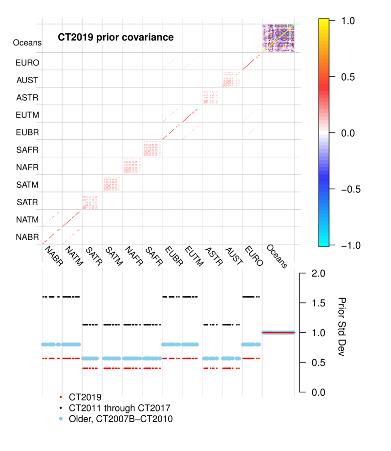
Figure 15: CT2019B prior covariance structure. The prior covariance
matrix (top panel) and the square root of diagonal members of this
matrix (bottom panel). Covariance matrix quantities are
dimensionless squared scaling factors, and the bottom panel is the
square root of this. Transcom land regions form the first 11 large
divisions on the axes here. As described in
Sec. 9, each of those regions contains 19
potential ecosystems. Correlations between similar ecosystems in
proximate Transcom regions are visible in North America (e.g. NABR
and NATM, the boreal and temperate North American regions) and
Eurasia. Within tropical Transcom regions, however, differing
ecosystems are assigned a non-zero prior covariance, which is
visible here as red block-like structures on the diagonal within,
for example, the South America Tropical (SATR) Transcom
region. Ocean regions have a more complicated covariance structure
that depends on which prior is used; the structure shown here is
that of the ocean inversion flux prior. The lower panel of this
diagram compares the on-diagonal elements of the prior covariance
matrix by plotting their square roots. The resulting standard
deviations are directly comparable to the percentages discussed in
section 3 above; 0.5 is equivalent to 50%. The retuning of the
covariance matrix for CT2019B's multiple-prior simulation (in red) is
made evident by also showing these values from previous
CarbonTracker releases in light blue and black.
While the correlation structure discussed above has remained fixed in
all CarbonTracker releases, we have been changing the overall
magnitude of the covariance matrix in an attempt to mitigate seasonal
biases in our simulated CO2 fields. Since those biases appear
mostly in comparison to measurement data over land, and also because
the annual cycle of CO2 in the atmosphere is dominated by the
terrestrial carbon cycle, we experimented by loosening the land prior
constraint. This is made evident in the "CT2011 through CT2017"
trace in the lower panel of Fig. 15. As it turns out,
these biases were mostly due to our original short assimilation window
length (Sec. 8.1.2) and the convective flux problem
discussed in Sec. 6.2. As a result, for CT2019B we were
able to scale back the land prior covariance. "L-curve" analysis
(Hansen, 1998) suggested that these covariances could be reduced
even from the original levels, and new values are shown in red in the
lower panel of Fig. 15.
8.3 Multiple prior models
In Bayesian estimation systems like CarbonTracker, there is a potential for bias from a flux prior to propagate through the inversion system to the final result. It is difficult to quantify this effect, and as a result it is generally considered a requirement that flux priors be unbiased. We cannot guarantee this for any of our prior fluxes, be they the prior estimates for terrestrial or oceanic exchange, or the presumed wildfire and fossil fuel emissions. In order to explicitly quantify the impact of prior bias on our solution, in CT2019B we present the average of two inversions using different priors. We have used two terrestrial flux priors (including two wildfire emissions estimates), two air-sea CO2 exchange priors, and two estimates of imposed fossil fuel emissions in a factorial design experiment. Whereas previous releases conducted 8 independent inversions exploring each unique combination of priors in a factorial design, we have determined that interactions between priors are negligible. Thus, the quantification of uncertainty due to prior selection can be explored using just two inversions, each using a unique set of priors. We present as a final result the mean flux between these two inversions and the atmospheric CO2 distribution resulting from applying these mean fluxes to our atmospheric transport model. Each of the priors is described in detail in its corresponding documentation section.8.3.1 Posterior uncertainties in CarbonTracker
The formal "internal" error estimates produced by CarbonTracker are unrealistically large. This is largely a result of the dynamical model that introduces a fresh prior covariance matrix with every new week entering the assimilation window. Uncertainties using the new 12-week assimilation window are smaller that those from previous CarbonTracker releases that used a much shorter five-week assimilation window. Uncertainties in CarbonTracker tend to increase as larger regions are considered; regional errors mostly just add in quadrature without any cancellation from dipole anticorrelation. Whereas many inversions yield smaller errors as the spatial extent of the region being considered increases, CarbonTracker acts in the opposite fashion. This is perhaps most obvious in the estimate of CarbonTracker's global annual surface flux of carbon dioxide. While CT2019B estimates a one-sigma error of about 2.7 PgC yr−1 on its global flux, this quantity is in actuality much more well-constrained. This is evident from CarbonTracker's excellent agreement both with observational estimates of atmospheric growth rate and with independent CO2 measurements. In CT2019B, our error estimates on optimized fluxes are smaller than those in previous releases. This is mainly due to the retuning of the land prior covariance discussed above. It should be noted that uncertainties presented for CT2019B take into account not only the "internal" flux uncertainty generated by a single inversion, but also the across-model "external" uncertainty representing the spread of the inversion models due to the choice of prior flux.9 Ecoregions in CarbonTracker
9.1 What are ecoregions?
Ecoregions are the actual scale on which CarbonTracker performs its optimization over land. Ecoregions are meant to represent large expanses of land within a given continent having similar ecosystem types, and are used to divide continent-scale regions into smaller domains for analysis. The ecosystem types use in CarbonTracker are derived from the Olson et al. (1992) vegetation classification (Table 5, Figure 16). We define an ecoregion as an ecosystem type within a given Transcom land region. There are 19 ecosystem types we extract from the Olson et al. (1992) system, and 11 Transcom land regions (Figure 17), so there are 11 × 19 = 209 possible ecoregions. However, not all ecosystem types are present in all Transcom regions, and the actual number of land ecoregions ends up being 126. Note on "Semitundra": this is a potentially misleading shorthand abbreviation for a collection of ecosystems comprising semi-desert, shrubs, steppe, and polar+alpine tundra. The "Semitundra" zones appearing in northern Africa where one expects to find the Sahara desert are not, of course, tundra environments. They are instead semi-desert zones.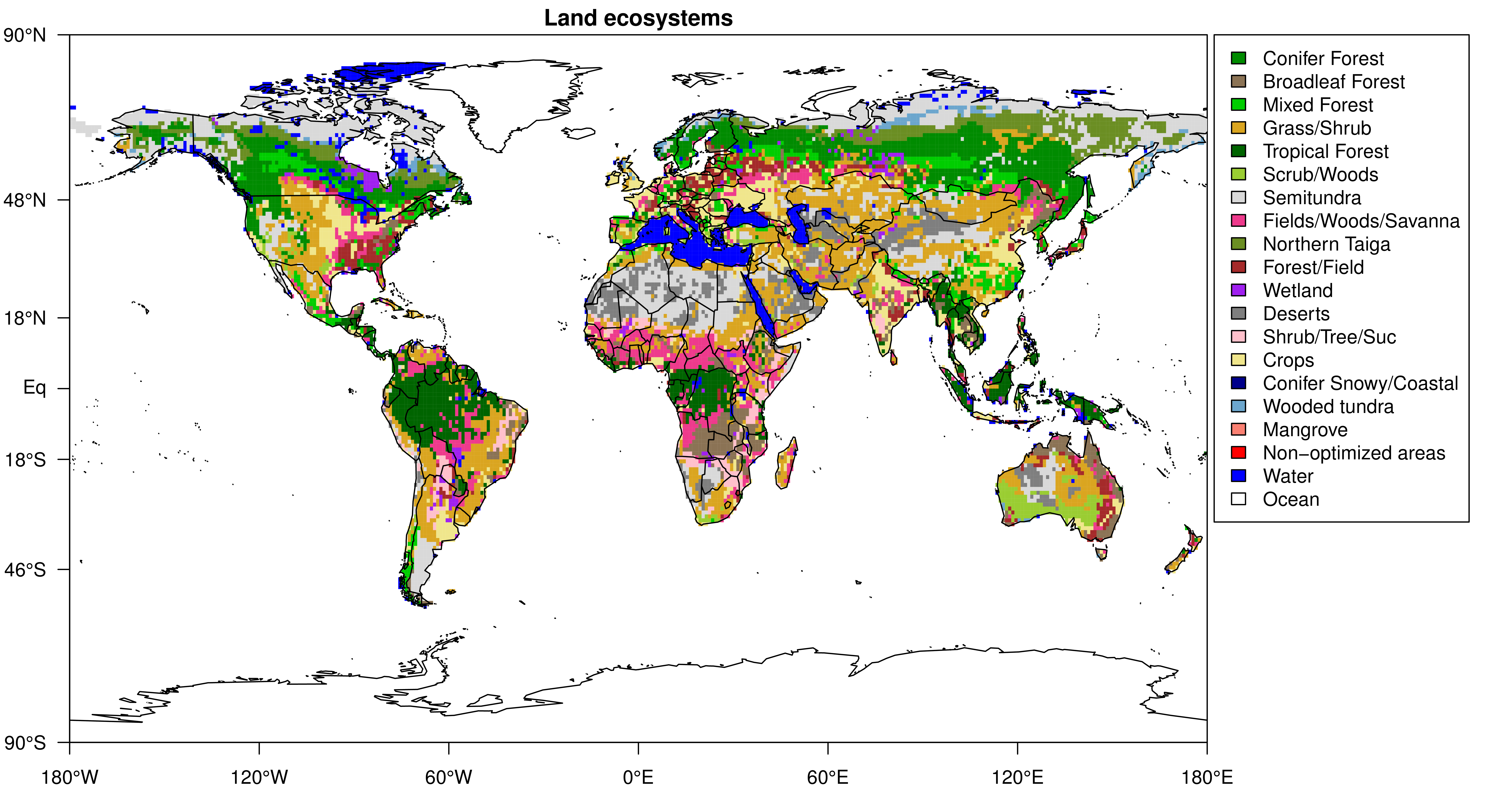
Figure 16: Global distribution of Olson ecosystem types.
| Ecosystem Type | North American Boreal | North American Temperate | ||
| Area (km2) | Percentage | Area (km2) | Percentage | |
| Conifer Forest | 2315376 | 22.9% | 1607291 | 14.0% |
| Broadleaf Forest | - | - | 269838 | 2.4% |
| Mixed Forest | 592291 | 5.9% | 930813 | 8.1% |
| Grass/Shrub | 53082 | 0.5% | 2515582 | 21.9% |
| Tropical Forest | - | - | 58401 | 0.5% |
| Scrub/Woods | - | - | 416520 | 3.6% |
| Semitundra | 3396292 | 33.6% | 866468 | 7.6% |
| Fields/Woods/Savanna | 29243 | 0.3% | 1020939 | 8.9% |
| Northern Taiga | 1658773 | 16.4% | - | - |
| Forest/Field | 61882 | 0.6% | 1243174 | 10.8% |
| Wetland | 322485 | 3.2% | 66968 | 0.6% |
| Deserts | - | - | 21934 | 0.2% |
| Shrub/Tree/Suc | - | - | 11339 | 0.1% |
| Crops | - | - | 1969912 | 17.2% |
| Conifer Snowy/Coastal | 41440 | 0.4% | 73437 | 0.6% |
| Wooded tundra | 360388 | 3.6% | 6643 | 0.1% |
| Mangrove | - | - | - | - |
| Non-optimized areas | - | - | - | - |
| Water | 1269485 | 12.6% | 384728 | 3.4% |
| Total | 10100736 | 100.0% | 11463986 | 100.0% |
Table 4: Ecosystem areas over the two Transcom regions covering North America.
9.2 Why use ecoregions?
A fundamental challenge to atmospheric inversions like CarbonTracker is that there are not enough observations to directly constrain fluxes at all times and in all places. It is therefore necessary to find a way to reduce the number of unknowns being estimated. Strategies to reduce the number of unknowns in problems like this one generally impose information from external sources. In CarbonTracker, we reduce the problem size both by estimating fluxes at the ecoregion scale, and by using a terrestrial biological model to give a first guess flux from the ecoregion. The model is also used to give the spatial and temporal distribution of CO2 flux within a region and week.9.3 Ecosystems within Transcom regions
Each Transcom land region (Figure 17) can contain up to 19 ecoregions.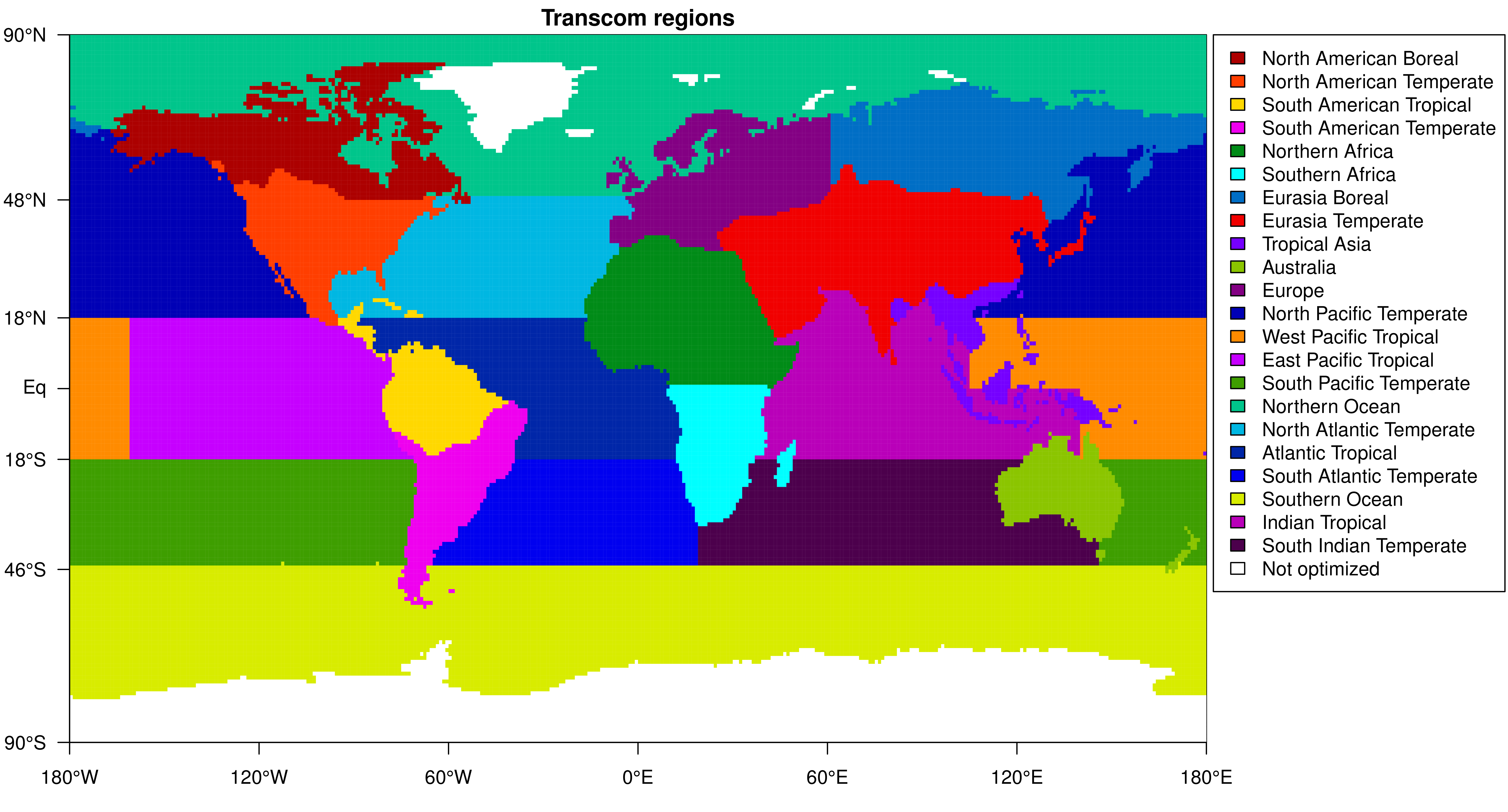
Figure 17: The 11 land regions and 11 ocean regions of the Transcom project, along with the unoptimized land areas in Greenland and Antarctica
.
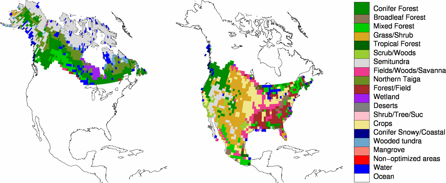
Figure 18: Ecoregions within the North American Boreal (left)
and North American Temperate (right) Transcom regions.
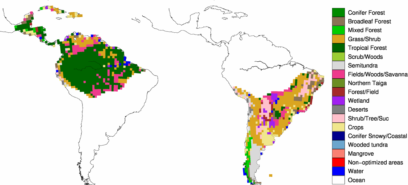
Figure 19: Ecoregions within the South American Tropical (left)
and South American Temperate (right) Transcom regions.
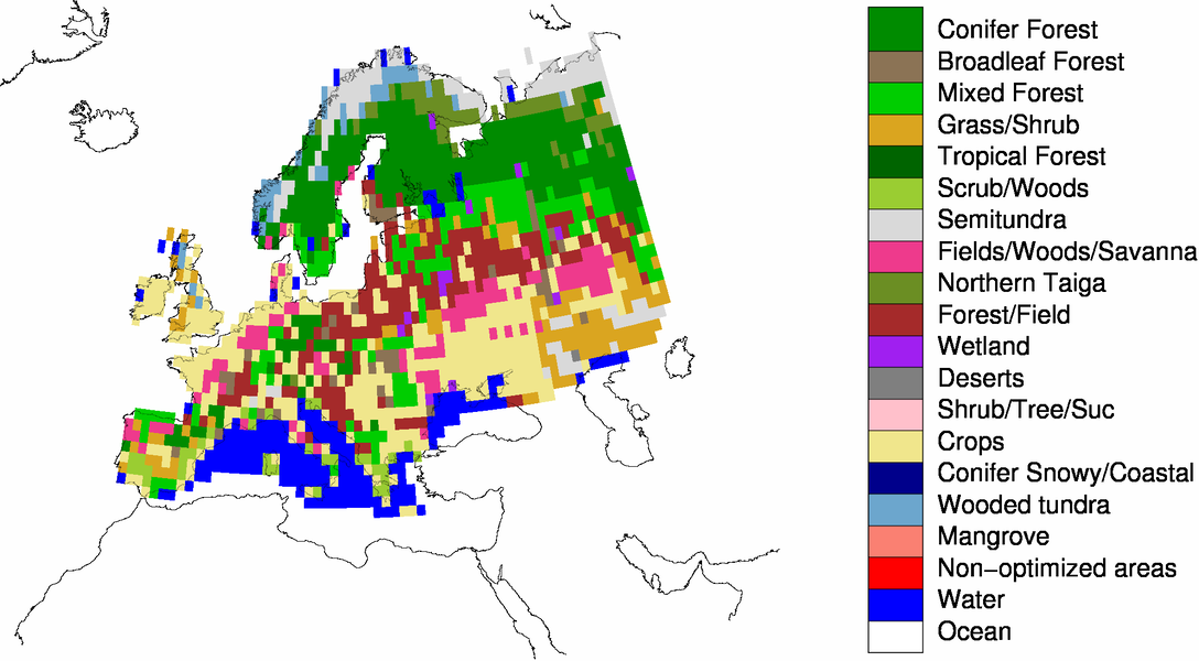
Figure 20: Ecoregions within the Europe Transcom region.
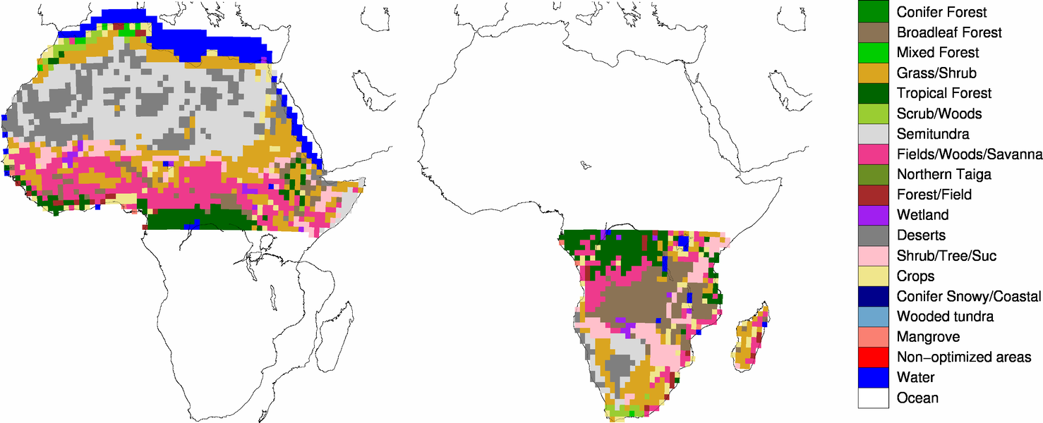
Figure 21: Ecoregions within the Northern Africa (left) and
Southern Africa (right) Transcom regions.
10 Resources and References
- Jim Randerson research group
- Global Fire Emissions Database (GFED) web page
- NASA GFED_CMS CASA project
- Olson ecosystem types
- Global Fire Emissions Database (GFED) web page
- GFED_CMS web page at NACP
- DOE Energy Information Administration (EIA)
- BP Statistical Review of World Energy
- EDGAR Database
- DMSP satellite nightlight data
- Centre for Air Transport and the Environment (CATE), AERO2k aviation emissions inventory
- NOAA Pacific Marine Environmental Laboratory
- Ocean Acidification
- ESRL Carbon Cycle Program
- WMO/GAW Report No. 168, 2006
References
- [Andres et al. 2011]
- R. J. Andres, J. S. Gregg, L. Losey, G. Marland, and T. A. Boden. Monthly, global emissions of carbon dioxide from fossil fuel consumption. Tellus B: Chemical and Physical Meteorology, 63 (3): 309-327, 2011.
- [Andres et al. 2014]
- R. J. Andres, T. A. Boden, and D. Higdon. A new evaluation of the uncertainty associated with CDIAC estimates of fossil fuel carbon dioxide emission. Tellus B: Chemical and Physical Meteorology, 66 (1): 23616, 2014.
- [Baker et al. 2006]
- D. F. Baker, R. M. Law, K. R. Gurney, P. Rayner, P. Peylin, A. S. Denning, P. Bousquet, L. Bruhwiler, Y. H. Chen, P. Ciais, I. Y. Fung, M. Heimann, J. John, T. Maki, S. Maksyutov, K. Masarie, M. Prather, B. Pak, S. Taguchi, and Z. Zhu. TransCom 3 CO2 inversion intercomparison: Impact of transport model errors on the interannual variability of regional CO2 fluxes, 1988-2003. Global Biogeochemical Cycles, 20 (1), 2006. GB1002.
- [Basu et al. 2016]
- S. Basu, J. B. Miller, and S. Lehman. Separation of biospheric and fossil fuel fluxes of CO2 by atmospheric inversion of CO2 and 14CO2 measurements: Observation system simulations. Atmos. Chem. Phys, 16 (9): 5665-5683, 2016.
- [Blasing et al. 2004]
- T. Blasing, G. Marland, and C. Broniak. Estimates of monthly CO2 emissions and associated 13C/12C values from fossil-fuel consumption in the USA (1981-2003). Carbon Dioxide Information Analysis Center, Oak Ridge National Laboratory, U.S. Department of Energy, Oak Ridge, Tenn., U.S.A., 2004. doi: 10.3334/CDIAC/ffe.001.
- [Boden et al. 2017]
- T. A. Boden, G. Marland, and R. J. Andres. Global, regional, and national fossil fuel CO2 emissions. Carbon Dioxide Information Analysis Center, Oak Ridge National Laboratory, U.S. Department of Energy, Oak Ridge, Tenn., U.S.A., 2017. doi: 10.3334/CDIAC/00001_V2017.
- [Boden et al. 2018]
- T. A. Boden, G. Marland, and R. J. Andres. Global, regional, and national fossil-fuel CO2 emissions. https://energy.appstate.edu/CDIAC, 2018.
- [British Petroleum 2019]
- British Petroleum. BP Statistical Review of World Energy. Number 68. BP p.l.c., London, 2019.
- [Bruhwiler et al. 2005]
- L. M. P. Bruhwiler, A. M. Michalak, W. Peters, D. F. Baker, and P. Tans. An improved Kalman smoother for atmospheric inversions. Atmospheric Chemistry and Physics, 5: 2691-2702, 2005. doi: https://doi.org/10.5194/acp-5-2691-2005.
- [Caldeira and Wickett 2003]
- K. Caldeira and M. E. Wickett. Anthropogenic carbon and ocean pH. Nature, 425 (6956): 365-365, 2003.
- [Cooperative Global Atmospheric Data Integration Project 2019]
- Cooperative Global Atmospheric Data Integration Project. Multi-laboratory compilation of atmospheric carbon dioxide data for the period 1957-2018; obspack_co2_1_GLOBALVIEWplus_v5.0_2019_08_12, 2019. http://dx.doi.org/10.25925/20190812, NOAA Earth System Research Laboratory, Global Monitoring Division.
- [European Commission 2011]
- European Commission. Emission database for global atmospheric research (EDGAR), release version 4.2. Technical report, Joint Research Centre (JRC)/Netherlands Environmental Assessment Agency (PBL), 2011. URL http://edgar.jrc.ec.europa.eu/.
- [Giglio et al. 2006]
- L. Giglio, G. R. van der Werf, J. T. Randerson, G. J. Collatz, and P. Kasibhatla. Global estimation of burned area using MODIS active fire observations. Atmospheric Chemistry and Physics, 6: 957-974, 2006.
- [Giglio et al. 2013]
- L. Giglio, J. T. Randerson, and G. R. van der Werf. Analysis of daily, monthly, and annual burned area using the fourth-generation global fire emissions database (GFED4). Journal of Geophysical Research: Biogeosciences, 118 (1): 317-328, 2013. doi: 10.1002/jgrg.20042. URL https://agupubs.onlinelibrary.wiley.com/doi/abs/10.1002/jgrg.20042.
- [Gloor et al. 2003]
- M. Gloor, N. Gruber, J. Sarmiento, C. L. Sabine, R. A. Feely, and C. Rödenbeck. A first estimate of present and preindustrial air-sea CO2 flux patterns based on ocean interior carbon measurements and models. Geophysical Research Letters, 30 (1): 10.1029/2002GL015594, 2003.
- [Gruber et al. 1996]
- N. Gruber, J. L. Sarmiento, and T. F. Stocker. An improved method for detecting anthropogenic CO2 in the oceans. Global Biogeochemical Cycles, 10 (4): 809-837, 1996.
- [Gurney et al. 2002]
- K. R. Gurney, R. M. Law, A. S. Denning, P. J. Rayner, D. Baker, P. Bousquet, L. Bruhwiler, Y.-H. Chen, P. Ciais, S. Fan, I. Y. Fung, M. Gloor, M. Heimann, K. Higuchi, J. John, T. Maki, S. Maksyutov, K. Masarie, P. Peylin, M. Prather, B. Pak, J. Randerson, J. L. Sarmiento, S. Taguchi, T. Takahashi, P. Tans, and C.-W. Yuen. Towards robust regional estimates of CO2 sources and sinks using atmospheric transport models. Nature, 415, 2002.
- [Hansen 1998]
- P. C. Hansen. Rank-deficient and discrete ill-posed problems: numerical aspects of linear inversion. SIAM, 1998.
- [Houtekamer and Mitchell 1998]
- P. L. Houtekamer and H. L. Mitchell. Data assimilation using an ensemble Kalman filter technique. Monthly Weather Review, 126 (3): 796-811, 1998. doi: 10.1175/1520-0493(1998)126<0796:DAUAEK>2.0.CO;2. URL https://doi.org/10.1175/1520-0493(1998)126<0796:DAUAEK>2.0.CO;2.
- [Jacobson et al. 2007]
- A. R. Jacobson, N. Gruber, J. L. Sarmiento, M. Gloor, and S. E. M. Fletcher. A joint atmosphere-ocean inversion for surface fluxes of carbon dioxide: I. methods and global-scale fluxes. Global Biogeochemical Cycles, 21 (GB1019), 2007.
- [Jacobson et al. 2020]
- A. R. Jacobson, K. N. Schuldt, J. B. Miller, T. Oda, P. Tans, A. Andrews, J. Mund, L. Ott, G. J. Collatz, T. Aalto, S. Afshar, K. Aikin, S. Aoki, F. Apadula, B. Baier, P. Bergamaschi, A. Beyersdorf, S. C. Biraud, A. Bollenbacher, D. Bowling, G. Brailsford, J. B. Abshire, G. Chen, H. Chen, L. Chmura, ..., and M. Zimnoch. CarbonTracker CT2019B. Model published by NOAA Global Monitoring Laboratory, 2020. URL https://gml.noaa.gov/ccgg/carbontracker/CT2019B/.
- [Kaminski et al. 2001]
- T. Kaminski, P. J. Rayner, M. Heimann, and I. G. Enting. On aggregation errors in atmospheric transport inversions. Journal of Geophysical Research-Atmospheres, 106 (D5): 4703-4715, 2001.
- [Krol et al. 2005]
- M. Krol, S. Houweling, B. Bregman, M. van den Broek, A. Segers, P. van Velthoven, W. Peters, F. Dentener, and P. Bergamaschi. The two-way nested global chemistry-transport zoom model TM5: algorithm and applications. Atmospheric Chemistry and Physics, 5: 417-432, 2005. URL http://www.atmos-chem-phys.net/5/417/2005/acp-5-417-2005.html.
- [Levitus et al. 2010]
- S. Levitus, R. A. Locarnini, T. P. Boyer, A. V. Mishonov, J. I. Antonov, H. E. Garcia, O. K. Baranova, M. M. Zweng, D. R. Johnson, and D. Seidov. World Ocean Atlas 2009. 2010.
- [Marland 2008]
- G. Marland. Uncertainties in accounting for CO2 from fossil fuels. Journal of Industrial Ecology, 12 (2): 136-139, 2008. doi: 10.1111/j.1530-9290.2008.00014.x. URL https://onlinelibrary.wiley.com/doi/abs/10.1111/j.1530-9290.2008.00014.x.
- [Mu et al. 2011]
- M. Mu, J. Randerson, G. Van der Werf, L. Giglio, P. Kasibhatla, D. Morton, G. Collatz, R. DeFries, E. Hyer, E. Prins, et al. Daily and 3-hourly variability in global fire emissions and consequences for atmospheric model predictions of carbon monoxide. Journal of Geophysical Research: Atmospheres, 116 (D24), 2011.
- [Nassar et al. 2013]
- R. Nassar, L. Napier-Linton, K. R. Gurney, R. J. Andres, T. Oda, F. R. Vogel, and F. Deng. Improving the temporal and spatial distribution of CO2 emissions from global fossil fuel emission data sets. Journal of Geophysical Research: Atmospheres, 118 (2): 917-933, 2013. doi: 10.1029/2012JD018196. URL https://agupubs.onlinelibrary.wiley.com/doi/abs/10.1029/2012JD018196.
- [Oda and Maksyutov 2011]
- T. Oda and S. Maksyutov. A very high-resolution (1 km x 1 km) global fossil fuel CO2 emission inventory derived using a point source database and satellite observations of nighttime lights. Atmospheric Chemistry and Physics, 11 (2): 543-556, 2011. doi: 10.5194/acp-11-543-2011. URL https://www.atmos-chem-phys.net/11/543/2011/.
- [Oda and Maksyutov 2015]
- T. Oda and S. Maksyutov. ODIAC fossil fuel CO2 emissions dataset. doi:10.17595/20170411.001, 2015.
- [Oda et al. 2018]
- T. Oda, S. Maksyutov, and R. J. Andres. The open-source data inventory for anthropogenic CO2, version 2016 (ODIAC2016): a global monthly fossil fuel CO2 gridded emissions data product for tracer transport simulations and surface flux inversions. Earth System Science Data, 10 (1): 87-107, 2018. doi: 10.5194/essd-10-87-2018. URL https://www.earth-syst-sci-data.net/10/87/2018/.
- [Olsen and Randerson 2004]
- S. C. Olsen and J. T. Randerson. Differences between surface and column atmospheric CO2 and implications for carbon cycle research. Journal of Geophysical Research-Atmospheres, 109 (D2), 2004.
- [Olson et al. 1992]
- J. Olson, J. Watts, and L. Allsion. Major world ecosystem complexes ranked by carbon in live vegetation: A database. Technical Report ORNL/CDIAC-134, NDP-017, 1992. URL http://cdiac.ornl.gov/epubs/ndp/ndp017/carbonbig.html.
- [Pacanowski and Gnanadesikan 1998]
- R. C. Pacanowski and A. Gnanadesikan. Transient response in a z-level ocean model that resolves topography with partial cells. Monthly Weather Review, 126: 3248-3270, 1998.
- [Patra et al. 2011]
- P. K. Patra, S. Houweling, M. Krol, P. Bousquet, D. Belikov, D. Bergmann, H. Bian, P. Cameron-Smith, M. P. Chipperfield, K. Corbin, et al. TransCom model simulations of CH4 and related species: linking transport, surface flux and chemical loss with CH4 variability in the troposphere and lower stratosphere. Atmospheric Chemistry and Physics, 11 (24): 12813-12837, 2011.
- [Peters et al. 2004]
- W. Peters, M. C. Krol, E. J. Dlugokencky, F. J. Dentener, P. Bergamaschi, G. Dutton, P. von Velthoven, J. B. Miller, L. Bruhwiler, and P. P. Tans. Toward regional-scale modeling using the two-way nested global model TM5: Characterization of transport using SF6. Journal of Geophysical Research-Atmospheres, 109 (D19), 2004. D19314.
- [Peters et al. 2005]
- W. Peters, J. Miller, J. Whitaker, A. Denning, A. Hirsch, M. Krol, D. Zupanski, L. Bruhwiler, and P. Tans. An ensemble data assimilation system to estimate CO2 surface fluxes from atmospheric trace gas observations. Journal of Geophysical Research-Atmospheres, 110: D24304, Jan 2005. doi: 10.1029/2005JD006157. D24304.
- [Potter et al. 1993]
- C. S. Potter, J. T. Randerson, C. B. Field, P. A. Matson, P. M. Vitousek, H. A. Mooney, and S. A. Klooster. Terrestrial ecosystem production - a process model-based on global satellite and surface data. Global Biogeochemical Cycles, 7 (4): 811-841, 1993.
- [Rasmussen 1991]
- L. Rasmussen. Piecewise integral splines of low degree. Computers & Geosciences, 17 (9): 1255-1263, 1991.
- [Sabine et al. 2004]
- C. L. Sabine, R. A. Feely, N. Gruber, R. M. Key, K. Lee, J. L. Bullister, R. Wanninkhof, C. S. Wong, D. W. R. Wallace, B. Tilbrook, F. J. Millero, T. H. Peng, A. Kozyr, T. Ono, and A. F. Rios. The oceanic sink for anthropogenic CO2. Science, 305 (5682): 367-371, 2004.
- [Sasakawa et al. 2010]
- M. Sasakawa, K. Shimoyama, T. Machida, N. Tsuda, H. Suto, M. Arshinov, D. Davydov, A. Fofonov, O. Krasnov, T. . Saeki, Y. Koyama, and S. Maksyutov. Continuous measurements of methane from a tower network over Siberia. Tellus B, 62 (5): 403-416, 2010.
- [Sasakawa et al. 2013]
- M. Sasakawa, T. Machida, N. Tsuda, M. Arshinov, D. Davydov, A. Fofonov, and O. Krasnov. Aircraft and tower measurements of CO2 concentration in the planetary boundary layer and the lower free troposphere over southern taiga in West Sib eria: Long-term records from 2002 to 2011. Journal of Geophysical Research, 118 (16): 9489-9498, 2013.
- [Schuh et al. 2019]
- A. E. Schuh, A. R. Jacobson, S. Basu, B. Weir, D. Baker, K. Bowman, F. Chevallier, S. Crowell, K. J. Davis, F. Deng, et al. Quantifying the impact of atmospheric transport uncertainty on CO2 surface flux estimates. Global Biogeochemical Cycles, 33 (4): 484-500, 2019.
- [Takahashi et al. 2002]
- T. Takahashi, S. C. Sutherland, C. Sweeney, A. P. N. Metzl, B. Tilbrook, N. Bates, R. Wanninkhof, R. A. Feely, C. Sabine, J. Olafsson, and Y. Nojiri. Global air-sea CO2 flux based on climatological surface ocean pCO2, and seasonal biological and temperature effects. Deep-Sea Research II, 49: 1601-1622, 2002.
- [Takahashi et al. 2009]
- T. Takahashi, S. C. Sutherland, R. Wanninkhof, C. Sweeney, R. A. Feely, D. W. Chipman, B. Hales, G. Friederich, F. Chavez, C. Sabine, et al. Climatological mean and decadal change in surface ocean pCO2, and net sea-air CO2 flux over the global oceans. Deep Sea Research Part II: Topical Studies in Oceanography, 56 (8-10): 554-577, 2009.
- [Thoning et al. 1989]
- K. W. Thoning, P. P. Tans, and W. D. Komhyr. Atmospheric carbon dioxide at Mauna Loa observatory. 2. Analysis of the NOAA GMCC data, 1974-1985. Journal of Geophysical Research-Atmospheres, 94: 8549-8565, Jan 1989.
- [van der Werf et al. 2003]
- G. van der Werf, J. Randerson, G. Collatz, and L. Giglio. Carbon emissions from fires in tropical and subtropical ecosystems. Global Change Biology, 9: 547-562, Jan 2003.
- [van der Werf et al. 2006]
- G. R. van der Werf, J. T. Randerson, L. Giglio, G. J. Collatz, P. S. Kasibhatla, and A. F. Arellano. Interannual variability in global biomass burning emissions from 1997 to 2004. Atmospheric Chemistry and Physics, 6: 3423-3441, Jan 2006.
- [van der Werf et al. 2017]
- G. R. van der Werf, J. T. Randerson, L. Giglio, T. T. van Leeuwen, Y. Chen, B. M. Rogers, M. Mu, M. J. E. van Marle, D. C. Morton, G. J. Collatz, R. J. Yokelson, and P. S. Kasibhatla. Global fire emissions estimates during 1997-2016. Earth System Science Data, 9 (2): 697-720, 2017. doi: 10.5194/essd-9-697-2017. URL https://www.earth-syst-sci-data.net/9/697/2017/.
- [Wanninkhof 1992]
- R. Wanninkhof. Relationship between wind-speed and gas-exchange over the ocean. Journal of Geophysical Research-Oceans, 97: 7373-7382, Jan 1992.
- [Whitaker and Hamill 2002]
- J. S. Whitaker and T. M. Hamill. Ensemble data assimilation without perturbed observations. Monthly Weather Review, 130 (7): 1913-1924, 2002.
File translated from TEX by TTH, version 4.04.
On 12 Nov 2020, 15:45.