
Information
Home FAQ Project Goals Documentation Collaborators TutorialResults
Fluxes Observations Evaluation Visualization DownloadGet Involved
Suggestions E-mail List Contact UsResources
How to Cite Version History Glossary References Bibliography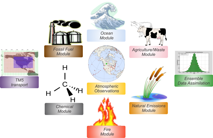
To learn more about a CarbonTracker component, click on one of the above images.
Or download the full PDF version for convenience.
TM5 Nested Transport
Introduction
The link between the observation of atmospheric trace constitutents in the air and their exchange at the Earth's surface, is their atmospheric transport: storm systems, cloud complexes, and various other types of weather, cause winds that transport atmospheric trace constituents around the world. As a result, local events like fires and fossil fuel emissions often impact remote locations. To simulate winds and weather, CarbonTracker uses sophisticated numerical models that are driven by the daily weather forecasts from specialized meteorological centers of the world. After accounting for any chemical loss, the influence of emissions and uptake in locations such as North America and Europe, are seen in our measurements, including places like the South Pole! Despite seeing the influence of emissions in our model, simulating the specific transport processes of atmospheric trace species remains a challenge. Not only is it difficult but it is also technologically expensive, costing almost 90% of the computer resources for CarbonTracker. To represent the atmospheric transport, Transport Model 5 (TM5) is used. This is a community-supported model whose development is shared among many scientific groups with different areas of expertise. TM5 is used for many applications other than CarbonTracker, including forecasting air-quality, studying the dispersion of aerosols in the tropics, tracking biomass burning plumes, and predicting pollution levels that future generations will have to deal with.
Detailed Description
TM5 is a global model with two-way nested grids. This means that using TM5, regions for which high-resolution simulations are desired, can be nested in a coarser grid spanning the global domain. The advantage to this approach is that transport simulations can be performed with a regional focus without the need for boundary conditions from other models. Further, this approach allows measurements outside the "zoom" domain to constrain regional fluxes in the data assimilation, and ensures that regional estimates are consistent with global constraints. TM5 is based on the predecessor model TM3, but has seen improvements in the advection scheme, vertical diffusion parameterization, and meteorological preprocessing of the wind fields (Krol et al., 2005).
The model is developed and maintained jointly by the Institute for Marine and Atmospheric Research Utrecht (IMAU, The Netherlands), the Joint Research Centre (JRC, Italy), the Royal Netherlands Meteorological Institute (KNMI, The Netherlands), and NOAA ESRL (USA).
In CarbonTracker, TM5 separately simulates advection, convection (deep and shallow), and vertical diffusion in the planetary boundary layer and free troposphere.

The winds which drive TM5 come from the European Center for Medium range Weather Forecast (ECMWF) operational forecast model. This "parent" model currently runs with ~25 km horizontal resolution and 60 layers in the vertical prior to 2006 (and 91 layers in the vertical from 2006 onwards). The carbon dioxide levels predicted by CarbonTracker do not feed back onto these predictions of winds.
For use in TM5, the ECMWF meteorological data are preprocessed into coarser grids. In CarbonTracker, TM5 is run at a global 3°x 2° resolution with a nested regional grid over North America at 1° x 1° resolution (Figure 1). TM5 runs at an external time step of three hours, but due to the symmetrical operator splitting and the refined resolution in nested grids, processes at the finest scale are repeated every 10 minutes. The vertical resolution of TM5 in CarbonTracker is 34 hybrid sigma-pressure levels (from 2006 onwards; 25 levels for 2000-2005). These levels are unevenly spaced, with more levels near the surface. Approximate heights of the mid-levels (in meters, with a surface pressure of 1012 hPa) are:
| Level | Height (m) | Level | Height (m) |
|---|---|---|---|
| 1 | 34.5 | 14 | 9076.6 |
| 2 | 111.9 | 15 | 10533.3 |
| 3 | 256.9 | 16 | 12108.3 |
| 4 | 490.4 | 17 | 13874.2 |
| 5 | 826.4 | 18 | 15860.1 |
| 6 | 1274.1 | 19 | 18093.2 |
| 7 | 1839.0 | 20 | 20590.0 |
| 8 | 2524.0 | 21 | 24247.3 |
| 9 | 3329.9 | 22 | 29859.6 |
| 10 | 4255.6 | 23 | 35695.0 |
| 11 | 5298.5 | 24 | 42551.5 |
| 12 | 6453.8 | 25 | 80000.0 |
| 13 | 7715.4 |